Tutorial for MIBI-TOF TNBC dataset
Need additional packages: scanpy seaborn plotly lifelines statannotations
Load the packages
[ ]:
%reload_ext autoreload
%autoreload 2

import os
import time
import scanpy as sc
import pandas as pd
import numpy as np
import anndata as ad
import seaborn as sns
import matplotlib.pyplot as plt
import matplotlib.patches as mpatches
from matplotlib.lines import Line2D

from Harmonics import *

import warnings
warnings.filterwarnings("ignore")

sc.settings.verbosity = 0
sc.settings.set_figure_params(dpi=50, dpi_save=500)

from matplotlib import rcParams
rcParams["figure.dpi"] = 50
rcParams["savefig.dpi"] = 500
rcParams['pdf.fonttype'] = 42
rcParams['svg.fonttype'] = 'none'
rcParams['ps.fonttype'] = 42
# rcParams['font.family'] = 'Arial'
rcParams['savefig.transparent'] = True
[2]:
data_dir = '../../../Data/Spatial/Proteomics/MIBI-TOF_TNBC_Keren2018/'
save_dir = '../../results/MIBI-TOF_TNBC_Keren2018/Harmonics/'
if not os.path.exists(save_dir):
    os.makedirs(save_dir)
Define the function to change p values to corresponding star representation, used to show the results of additional tests implemented in Harmonics
[3]:
def p2stars(p):
    if p < 0.001:
        return '***'
    elif p < 0.01:
        return '**'
    elif p < 0.05:
        return '*'
    else:
        return ''
Load dataset
Cells with unidentitied type are filtered out.
Use the cold group as the control group and use the mix and compartmentalized group as the case group
[4]:
cold_group = [15, 19, 22, 24, 25, 26]  # 6
mixed_group = [1, 2, 7, 8, 11, 12, 13, 14, 17, 18, 20, 21, 23, 27, 29, 31, 33, 38, 39]  # 19
compartmentalized_group = [3, 4, 5, 6, 9, 10, 16, 28, 32, 34, 35, 36, 37, 40, 41]  #15

adata_list = []
slice_name_list = []
cond_list = []
cond_name_list = []
for i in range(1, 42):
    if i == 30: continue
    adata = ad.read_h5ad(data_dir + f'TNBC_p{i}.h5ad')
    adata = adata[adata.obs['all_group_name'] != 'Unidentified', :].copy()
    if i in cold_group:
        adata_list.append(adata)
        slice_name_list.append(f'p{i}')
    else:
        cond_list.append(adata)
        cond_name_list.append(f'p{i}')
Run model
Instantiate Harmonics
[5]:
model = Harmonics_Model(adata_list,
                        slice_name_list,
                        cond_list=cond_list,
                        cond_name_list=cond_name_list,
                        concat_label='slice_name',  # default
                        proportion_label=None,  # default
                        seed=1234,  # default
                        parallel=True,  # default
                        verbose=True,  # default
                        )
Control set comprises 6 slices, 22748 cells/spots in total.
Condition set comprises 34 slices, 173205 cells/spots in total.
Preprocess the data (Generating the connection graph and calculating neighborhood cell type destribution for cells)
[6]:
model.preprocess(ct_key='all_group_name',
                 spatial_key='spatial',  # default
                 method='joint',  # default
                 n_step=3,  # default
                 n_neighbors=20,  # default
                 cut_percentage=99,  # default
                 )
Generating Delaunay neighbor graph...
100%|██████████| 40/40 [00:01<00:00, 29.43it/s]
All done!

Performing graph completion...
100%|██████████| 40/40 [00:11<00:00, 3.44it/s]
All done!

The cell types of interest are:
B
CD3 T
CD4 T
CD8 T
DC
DC/Mono
Endothelial
Keratin+ tumor
Macrophages
Mesenchymal like
Mono/Neu
NK
Neutrophils
Other immune
Tregs
Tumor

Generating one-hot matrix...
100%|██████████| 40/40 [00:00<00:00, 282.63it/s]
All done!

Dataset comprises 16 cell types.

Calculating cell type distribution for microenvironments...
Microenvironments comprise 40.06 cells/spots on average.
Minimum: 20, Maximum: 81
Perform overclustered initialization on the cell type distributions of cell neighborhoods for the control group. Resulting in Qmax niches. The distributions of niches are also computed.
[7]:
model.initialize_clusters(dim_reduction=True,  # default
                          explained_var=None,  # default
                          n_components=None,  # default
                          n_components_max=100,  # default
                          standardize=True,  # default
                          method='kmeans',  # default
                          Qmax=20,
                          )
Performing dimension reduction...
Returning 16 principal components.

Initializing niches...
20 initial niches defined.
Perform hierarchical distribution matching for the control group to reduce the niche number to no less than Qmin. This step results in niche assignment under a sequence of different niche numbers (usually from Qmax to Qmin).
[ ]:
model.hier_dist_match(assign_metric='jsd',  # default
                      weighted_merge=True,  # default
                      max_iters=100,  # default
                      tol=1e-4,  # default
                      test_kmeans=False,  # default
                      Qmin=2,  # default
                      )
Starting from 20 cell niches...

Assigning cells to cell niche...
Current state: [0, 1, 2, 3, 4, 5, 6, 7, 8, 9, 10, 11, 12, 13, 14, 15, 16, 17, 18, 19]
100%|██████████| 100/100 [00:02<00:00, 40.75it/s]
Unconverged at iteration 100!
13 cell niches left.
Merging cell niche 1 and cell niche 4...
Done!

Assigning cells to cell niche...
Current state: [0, 1, 3, 5, 8, 9, 12, 13, 15, 16, 17, 19]
100%|██████████| 100/100 [00:01<00:00, 60.75it/s]
Unconverged at iteration 100!
11 cell niches left.
Merging cell niche 1 and cell niche 3...
Done!

Assigning cells to cell niche...
Current state: [0, 1, 5, 8, 9, 12, 13, 15, 17, 19]
100%|██████████| 100/100 [00:01<00:00, 62.57it/s]
Unconverged at iteration 100!
10 cell niches left.
Merging cell niche 8 and cell niche 1...
Done!

Assigning cells to cell niche...
Current state: [0, 5, 8, 9, 12, 13, 15, 17, 19]
100%|██████████| 100/100 [00:01<00:00, 64.82it/s]
Unconverged at iteration 100!
9 cell niches left.
Merging cell niche 12 and cell niche 8...
Done!

Assigning cells to cell niche...
Current state: [0, 5, 9, 12, 13, 15, 17, 19]
38%|███▊ | 38/100 [00:00<00:00, 63.01it/s]
Distribution of cell niches (centers) converge at iteration 39.
8 cell niches left.
Merging cell niche 12 and cell niche 17...
Done!

Assigning cells to cell niche...
Current state: [0, 5, 9, 12, 13, 15, 19]
52%|█████▏ | 52/100 [00:00<00:00, 65.62it/s]
Distribution of cell niches (centers) converge at iteration 53.
7 cell niches left.
Merging cell niche 15 and cell niche 12...
Done!

Assigning cells to cell niche...
Current state: [0, 5, 9, 13, 15, 19]
100%|██████████| 100/100 [00:01<00:00, 65.35it/s]
Unconverged at iteration 100!
6 cell niches left.
Merging cell niche 15 and cell niche 5...
Done!

Assigning cells to cell niche...
Current state: [0, 9, 13, 15, 19]
41%|████ | 41/100 [00:00<00:00, 67.87it/s]
Strictly converge at iteration 42.
5 cell niches left.
Merging cell niche 15 and cell niche 19...
Done!

Assigning cells to cell niche...
Current state: [0, 9, 13, 15]
8%|▊ | 8/100 [00:00<00:01, 61.30it/s]
Distribution of cell niches (centers) converge at iteration 9.
4 cell niches left.
Merging cell niche 13 and cell niche 9...
Done!

Assigning cells to cell niche...
Current state: [0, 13, 15]
7%|▋ | 7/100 [00:00<00:01, 69.65it/s]
Distribution of cell niches (centers) converge at iteration 12.
11%|█ | 11/100 [00:00<00:01, 63.21it/s]
3 cell niches left.
Merging cell niche 15 and cell niche 0...
Done!

Assigning cells to cell niche...
Current state: [13, 15]
20%|██ | 20/100 [00:00<00:01, 68.37it/s]
Distribution of cell niches (centers) converge at iteration 21.
2 cell niches left.
Niche count no more than 2.

Finished!
Automatically define the most appropriate number of basic cell niches based on minJSD score for the control group. The results are saved in .obs[niche_key]
[9]:
adata_list, adata_concat = model.select_solution(n_niche=None,  # default
                                                 niche_key='niche_label',  # default
                                                 auto=True,  # default
                                                 metric='jsd_v2',  # default
                                                 threshold=0.1,  # default
                                                 return_adata=True,  # default
                                                 plot=True,  # default
                                                 save=False,  # default
                                                 fig_size=None,  # default
                                                 save_dir=save_dir,
                                                 file_name=f'score_vs_nichecount_basic.pdf',
                                                 )
Automatically selecting best solution...
100%|██████████| 100/100 [00:00<00:00, 348.97it/s]
100%|██████████| 100/100 [00:00<00:00, 404.82it/s]
100%|██████████| 100/100 [00:00<00:00, 379.46it/s]
100%|██████████| 100/100 [00:00<00:00, 494.99it/s]
100%|██████████| 100/100 [00:00<00:00, 591.65it/s]
100%|██████████| 100/100 [00:00<00:00, 621.04it/s]
100%|██████████| 100/100 [00:00<00:00, 706.65it/s]
100%|██████████| 100/100 [00:00<00:00, 666.59it/s]
100%|██████████| 100/100 [00:00<00:00, 865.71it/s]
100%|██████████| 100/100 [00:00<00:00, 985.12it/s]
100%|██████████| 100/100 [00:00<00:00, 1069.42it/s]
Suggested range of niche count is from 5 to 6.
Recommended number of niches are [6]
Selecting 6 niches as the best solution.
Done!
Perform overclustered initialization on the cell type distributions of cell neighborhoods for the case group. Resulting in Rmax new niches. The distributions of new niches are also computed.
[10]:
model.initialize_clusters_cond(assign_metric='jsd',  # default
                               threshold=0.1,  # default
                               min_cell_per_niche=100,  # default
                               dim_reduction=True,  # default
                               explained_var=None,  # default
                               n_components=None,  # default
                               n_components_max=100,  # default
                               standardize=True,  # default
                               method='kmeans',  # default
                               Rmax=10,  # default
                               )
Assigning cells to fixed niches...
67789 out of 173205 cells are assigned to fixed niches.

Performing dimension reduction...
Returning 16 principal components.

Initializing niches...
10 new niches defined.
Perform hierarchical distribution matching for the case group to reduce the niche number to 0. This step results in niche assignment under a sequence of different niche numbers (usually from Rmax to 0).
[11]:
model.hier_dist_match_cond(assign_metric='jsd',  # default
                           weighted_merge=True,  # default
                           max_iters=100,  # default
                           tol=1e-4,  # default
                           )
Starting from 10 new cell niches...

Assigning cells to cell niche...
Current state: [0, 1, 2, 3, 4, 5, 6, 7, 8, 9, 10, 11, 12, 13, 14, 15]
35%|███▌ | 35/100 [00:05<00:09, 6.78it/s]
Distribution of cell niches (centers) converge at iteration 36.
10 new cell niches left.
Merging new cell niche 14 and new cell niche 8...
Done!

Assigning cells to cell niche...
Current state: [0, 1, 2, 3, 4, 5, 6, 7, 9, 10, 11, 12, 13, 14, 15]
94%|█████████▍| 94/100 [00:14<00:00, 6.68it/s]
Distribution of cell niches (centers) converge at iteration 95.
9 new cell niches left.
Merging new cell niche 14 and new cell niche 6...
Done!

Assigning cells to cell niche...
Current state: [0, 1, 2, 3, 4, 5, 7, 9, 10, 11, 12, 13, 14, 15]
73%|███████▎ | 73/100 [00:11<00:04, 6.55it/s]
Distribution of cell niches (centers) converge at iteration 74.
8 new cell niches left.
Merging new cell niche 14 and new cell niche 7...
Done!

Assigning cells to cell niche...
Current state: [0, 1, 2, 3, 4, 5, 9, 10, 11, 12, 13, 14, 15]
19%|█▉ | 19/100 [00:02<00:12, 6.53it/s]
Distribution of cell niches (centers) converge at iteration 20.
7 new cell niches left.
Merging new cell niche 12 and new cell niche 14...
Done!

Assigning cells to cell niche...
Current state: [0, 1, 2, 3, 4, 5, 9, 10, 11, 12, 13, 15]
14%|█▍ | 14/100 [00:02<00:13, 6.59it/s]
Distribution of cell niches (centers) converge at iteration 15.
6 new cell niches left.
Merging new cell niche 12 and new cell niche 15...
Done!

Assigning cells to cell niche...
Current state: [0, 1, 2, 3, 4, 5, 9, 10, 11, 12, 13]
56%|█████▌ | 56/100 [00:07<00:06, 7.23it/s]
Distribution of cell niches (centers) converge at iteration 57.
5 new cell niches left.
Merging new cell niche 12 and new cell niche 9...
Done!

Assigning cells to cell niche...
Current state: [0, 1, 2, 3, 4, 5, 10, 11, 12, 13]
10%|█ | 10/100 [00:01<00:13, 6.78it/s]
Distribution of cell niches (centers) converge at iteration 11.
4 new cell niches left.
Merging new cell niche 12 and new cell niche 13...
Done!

Assigning cells to cell niche...
Current state: [0, 1, 2, 3, 4, 5, 10, 11, 12]
21%|██ | 21/100 [00:02<00:10, 7.44it/s]
Distribution of cell niches (centers) converge at iteration 22.
3 new cell niches left.
Merging new cell niche 11 and new cell niche 12...
Done!

Assigning cells to cell niche...
Current state: [0, 1, 2, 3, 4, 5, 10, 11]
18%|█▊ | 18/100 [00:02<00:10, 7.72it/s]
Distribution of cell niches (centers) converge at iteration 19.
2 new cell niches left.
Merging new cell niche 11 into basic cell niche 1...
Done!

Assigning cells to cell niche...
Current state: [0, 1, 2, 3, 4, 5, 10]
8%|▊ | 8/100 [00:00<00:11, 8.08it/s]
Distribution of cell niches (centers) converge at iteration 9.
1 new cell niches left.
Merging new cell niche 10 into basic cell niche 1...
Done!

Assigning cells to cell niche...
Current state: [0, 1, 2, 3, 4, 5]
No new cell niche, all cells assigned to basic niches.
0 new cell niches left.
No new cell niche left.

Finished!
Automatically define the most appropriate number of condition-specific niches based on minJSD score for the case group. The results of niche assignments are saved in .obs[niche_key] and .obs[csn_label]. All basic cell niches are named “basic” in .obs[csn_label] and condition-specific niches start with a prefix “R”.
[12]:
cond_list, cond_concat = model.select_solution_cond(n_csn=None,  # default
                                                    niche_key='niche_label',  # default
                                                    csn_key='csn_label',  # default
                                                    auto=True,  # default
                                                    metric='jsd_v2',  # default
                                                    threshold=0.1,  # default
                                                    return_adata=True,  # default
                                                    plot=True,  # default
                                                    save=False,  # default
                                                    fig_size=None,  # default
                                                    save_dir=save_dir,
                                                    file_name='score_vs_nichecount_cond.pdf',
                                                    )
Automatically selecting best solution...
100%|██████████| 100/100 [00:00<00:00, 231.25it/s]
100%|██████████| 100/100 [00:00<00:00, 232.76it/s]
100%|██████████| 100/100 [00:00<00:00, 261.93it/s]
100%|██████████| 100/100 [00:00<00:00, 247.27it/s]
100%|██████████| 100/100 [00:00<00:00, 249.47it/s]
100%|██████████| 100/100 [00:00<00:00, 266.48it/s]
100%|██████████| 100/100 [00:00<00:00, 271.80it/s]
100%|██████████| 100/100 [00:00<00:00, 352.75it/s]
100%|██████████| 100/100 [00:00<00:00, 382.92it/s]
100%|██████████| 100/100 [00:00<00:00, 573.89it/s]
Suggested range of condition specific niche count is from 4 to 5.
Recommended number of condition specific niches are [5]
Selecting 5 new niches as the best solution.
Done!
Save and reload the results
[ ]:
adata_concat.uns['ct_name'] = list(adata_concat.uns['ct2idx'].keys())
adata_concat.uns['ct_idx'] = list(adata_concat.uns['ct2idx'].values())
del adata_concat.uns['ct2idx'], adata_concat.uns['idx2ct']
adata_concat.write_h5ad(save_dir + 'Harmonics_basic_result_0.h5ad')

cond_concat.uns['ct_name'] = list(cond_concat.uns['ct2idx'].keys())
cond_concat.uns['ct_idx'] = list(cond_concat.uns['ct2idx'].values())
del cond_concat.uns['ct2idx'], cond_concat.uns['idx2ct']
cond_concat.write_h5ad(save_dir + 'Harmonics_cond_result_0.h5ad')
[14]:
adata_concat = ad.read_h5ad(save_dir + 'Harmonics_basic_result_0.h5ad')
adata_concat.uns['ct2idx'] = dict(zip(adata_concat.uns['ct_name'], adata_concat.uns['ct_idx']))
adata_concat.uns['idx2ct'] = dict(zip(adata_concat.uns['ct_idx'], adata_concat.uns['ct_name']))
cond_concat = ad.read_h5ad(save_dir + 'Harmonics_cond_result_0.h5ad')
cond_concat.uns['ct2idx'] = dict(zip(cond_concat.uns['ct_name'], cond_concat.uns['ct_idx']))
cond_concat.uns['idx2ct'] = dict(zip(cond_concat.uns['ct_idx'], cond_concat.uns['ct_name']))

for i, slice_name in enumerate(slice_name_list):
    adata = adata_concat[adata_concat.obs['slice_name'] == slice_name, :].copy()
    adata_list[i] = adata
for i, slice_name in enumerate(cond_name_list):
    adata = cond_concat[cond_concat.obs['slice_name'] == slice_name, :].copy()
    cond_list[i] = adata
[15]:
adata_concat_new = adata_concat.copy()
cond_concat_new = cond_concat.copy()
adata_concat_new, cond_concat_new
[15]:
(AnnData object with n_obs × n_vars = 22748 × 36
     obs: 'SampleID', 'cellLabelInImage', 'cellSize', 'tumorYN', 'group_name', 'immuneGroup_name', 'all_group_name', 'sample_types', 'slice_name', 'celltype_idx', 'n_neighbors', 'niche_label_13', 'niche_label_11', 'niche_label_10', 'niche_label_9', 'niche_label_8', 'niche_label_7', 'niche_label_6', 'niche_label_5', 'niche_label_4', 'niche_label_3', 'niche_label_2', 'niche_label_jsd_v2', 'niche_label_jsd', 'niche_label_fmi', 'niche_label_ari', 'niche_label_nmi', 'niche_label_asw', 'niche_label_js_asw', 'niche_label_fisher', 'niche_label_chi', 'niche_label_dbi', 'niche_label_dass_mean', 'niche_label_dass_min', 'niche_label_dafisher', 'niche_label_dachi', 'niche_label_0.09', 'niche_label_0.11', 'niche_label'
     uns: 'ct_idx', 'ct_name', 'niche_cell_count', 'niche_dist', 'niche_label_summary', 'score_dict', 'ct2idx', 'idx2ct'
     obsm: 'micro_dist', 'onehot', 'spatial',
 AnnData object with n_obs × n_vars = 173205 × 36
     obs: 'SampleID', 'cellLabelInImage', 'cellSize', 'tumorYN', 'group_name', 'immuneGroup_name', 'all_group_name', 'sample_types', 'slice_name', 'celltype_idx', 'n_neighbors', 'niche_label_10', 'csn_label_10', 'niche_label_9', 'csn_label_9', 'niche_label_8', 'csn_label_8', 'niche_label_7', 'csn_label_7', 'niche_label_6', 'csn_label_6', 'niche_label_5', 'csn_label_5', 'niche_label_4', 'csn_label_4', 'niche_label_3', 'csn_label_3', 'niche_label_2', 'csn_label_2', 'niche_label_1', 'csn_label_1', 'niche_label_0', 'csn_label_0', 'niche_label_jsd_v2', 'csn_label_jsd_v2', 'niche_label_jsd', 'csn_label_jsd', 'niche_label_fmi', 'csn_label_fmi', 'niche_label_ari', 'csn_label_ari', 'niche_label_nmi', 'csn_label_nmi', 'niche_label_asw', 'csn_label_asw', 'niche_label_js_asw', 'csn_label_js_asw', 'niche_label_fisher', 'csn_label_fisher', 'niche_label_chi', 'csn_label_chi', 'niche_label_dbi', 'csn_label_dbi', 'niche_label_dass_mean', 'csn_label_dass_mean', 'niche_label_dass_min', 'csn_label_dass_min', 'niche_label_dafisher', 'csn_label_dafisher', 'niche_label_dachi', 'csn_label_dachi', 'niche_label_0.09', 'csn_label_0.09', 'niche_label_0.11', 'csn_label_0.11', 'niche_label', 'csn_label'
     uns: 'ct_idx', 'ct_name', 'niche_cell_count', 'niche_dist', 'niche_label_summary', 'score_dict', 'ct2idx', 'idx2ct'
     obsm: 'micro_dist', 'onehot', 'spatial')
Plot the results
[16]:
tumor_color_dict = {f'{i}': sns.color_palette()[i] for i in range(2)}

niches = cond_concat_new.uns['niche_label_summary']
niche_colors = ['#1f77b4', '#ff7f0e', '#279e68', '#d62728', '#ffbb78', '#8c564b',
                '#aa40fc', '#b5bd61', '#aec7e8',  '#17becf', '#e377c2']
niche_color_dict = {niches[k]: niche_colors[k] for k in range(len(niches))}

n_basic_niches = len(adata_concat_new.uns['niche_label_summary'])
csns = [f'R{int(label)-n_basic_niches}' for label in niches[n_basic_niches:]]
csn_color_dict = {csns[k]: niche_colors[k+n_basic_niches] for k in range(len(csns))}
csn_color_dict['basic'] = '#d3d3d3'

celltypes = ['B', 'CD3 T', 'CD4 T', 'CD8 T', 'DC', 'DC/Mono', 'Endothelial', 'Keratin+ tumor', 'Macrophages', 'Mesenchymal like',
             'Mono/Neu', 'NK', 'Neutrophils', 'Other immune', 'Tregs', 'Tumor']#, 'Unidentified']
ct_colors = ['#1f77b4', '#ff7f0e', '#d62728', '#279e68', '#aa40fc', '#8c564b', '#e377c2', '#b5bd61', '#17becf', '#aec7e8',
             '#ffbb78', '#98df8a', '#ff9896', '#c5b0d5', '#c49c94', '#f7b6d2']#, '#d3d3d3']
ct_color_dict = {celltypes[k]: ct_colors[k] for k in range(len(celltypes))}
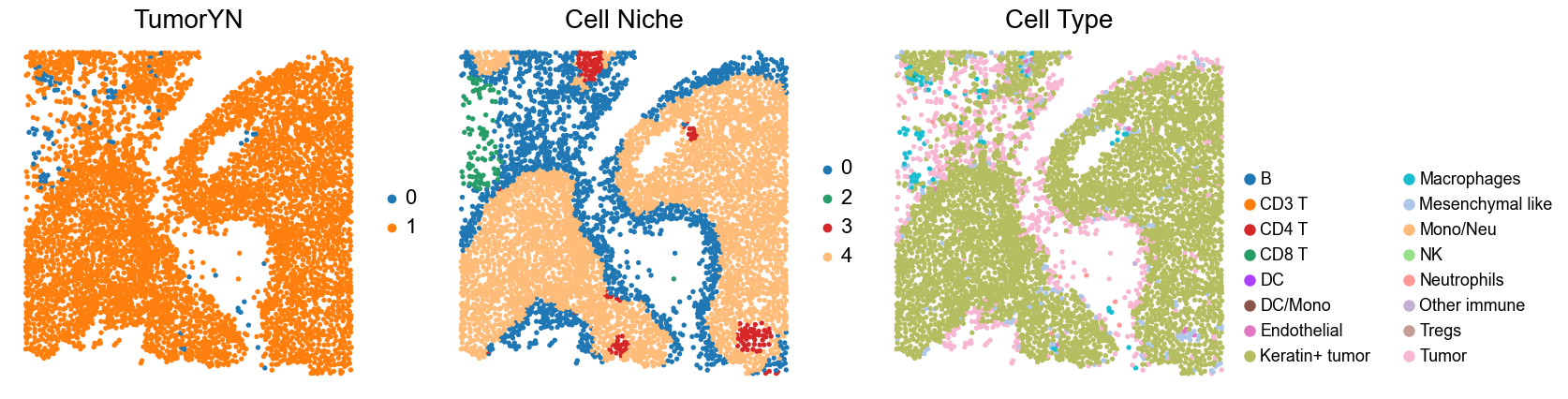
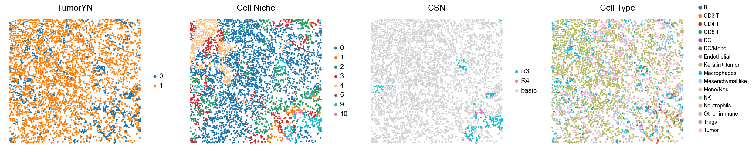
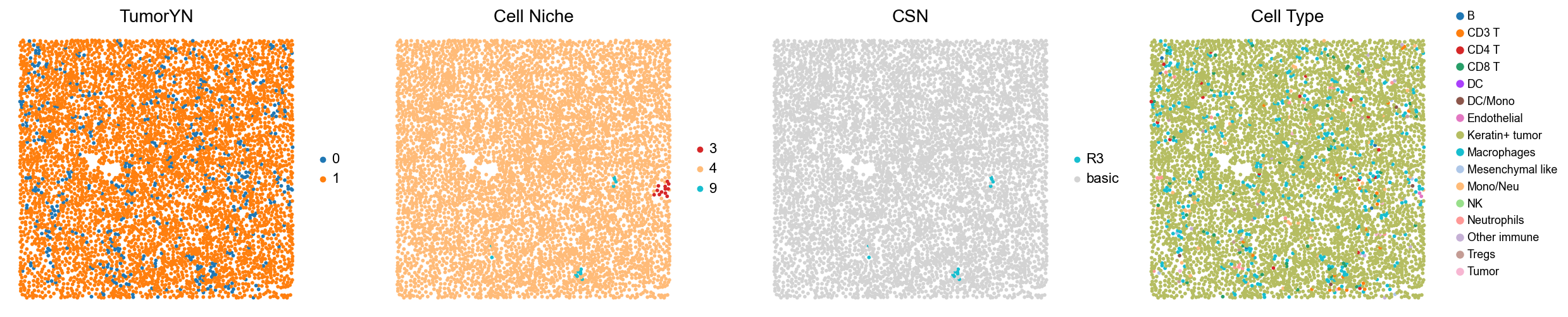
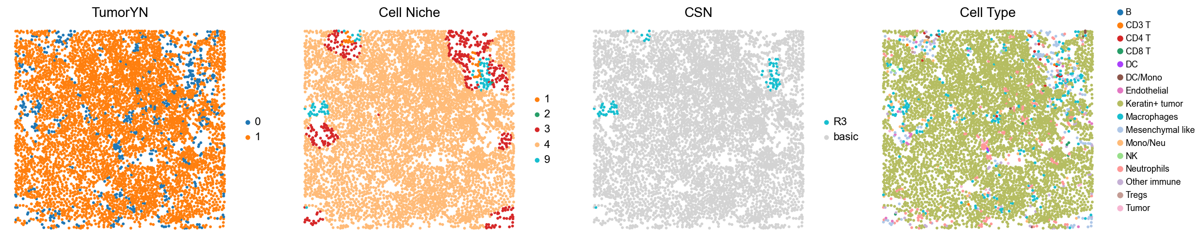
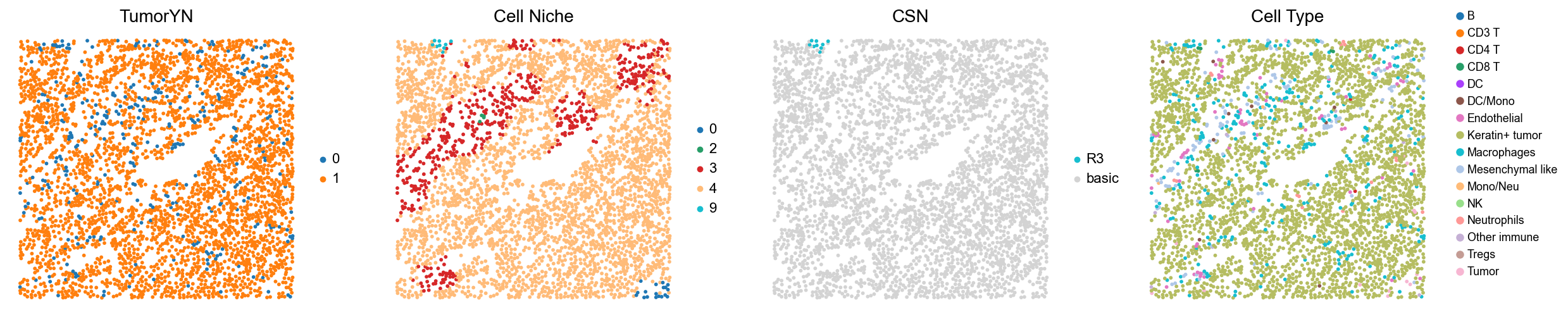
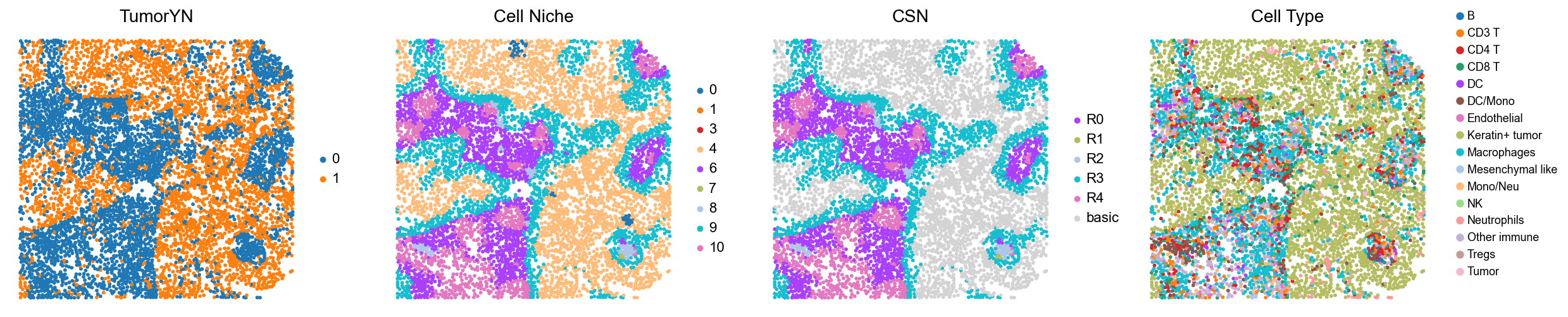
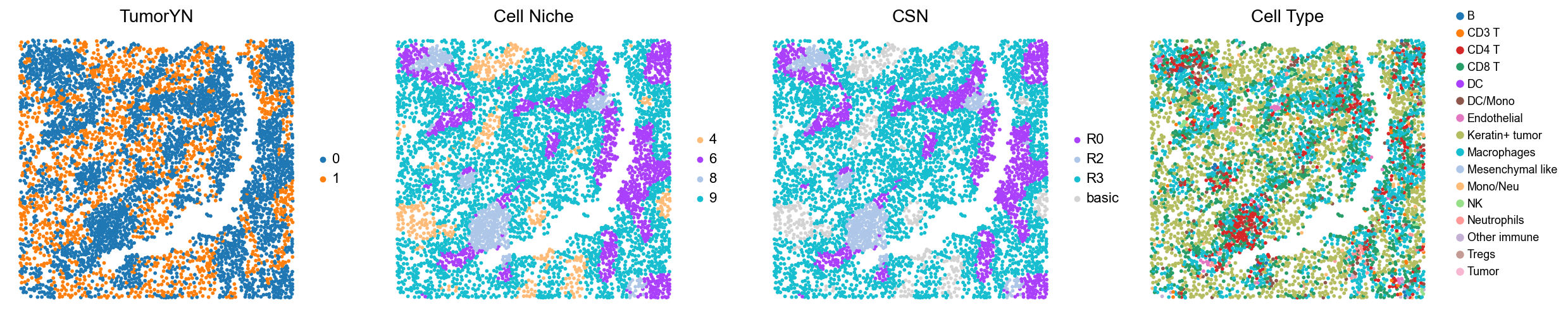
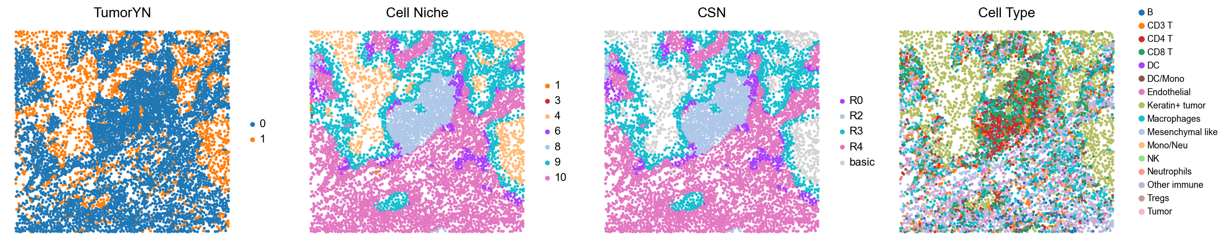
Control group (cold group)
[17]:
for i in range(len(cold_group)):

    print(f'p{cold_group[i]}')
    adata = adata_concat_new[adata_concat_new.obs['slice_name'] == f'p{cold_group[i]}', :].copy()

    fig, axes = plt.subplots(1, 3, figsize=(17, 4.5))

    sc.pl.embedding(adata, basis='spatial', color='tumorYN', palette=tumor_color_dict,
                    ax=axes[0], s=60, show=False, frameon=False, title='TumorYN', legend_fontsize=16)
    axes[0].set_title('TumorYN', fontsize=20)

    sc.pl.embedding(adata, basis='spatial', color='niche_label', palette=niche_color_dict,
                    ax=axes[1], s=60, show=False, frameon=False, title='Cell Niche', legend_fontsize=16)
    axes[1].set_title('Cell Niche', fontsize=20)

    sc.pl.embedding(adata, basis='spatial', color='all_group_name', palette=ct_color_dict,
                    ax=axes[2], s=60, show=False, frameon=False, title='Cell Type', legend_fontsize=16)
    axes[2].set_title('Cell Type', fontsize=20)

    ct_legend_elements = [
        Line2D([0], [0], marker='o', color='w', label=label,
            markerfacecolor=color, markersize=10)
        for label, color in ct_color_dict.items()
    ]
    axes[2].legend(handles=ct_legend_elements, loc=(1.0, 0.05), frameon=False, ncol=2)
    axes[2].axis('off')

    plt.tight_layout()
    plt.show()
p15
p19
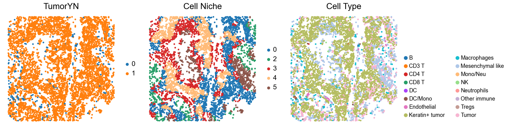
p22
p24
p25
p26
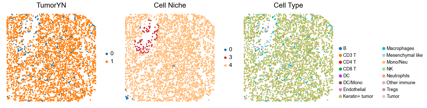
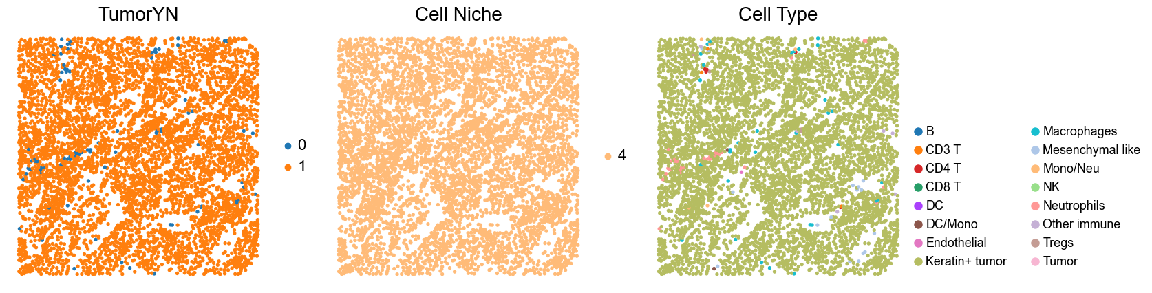
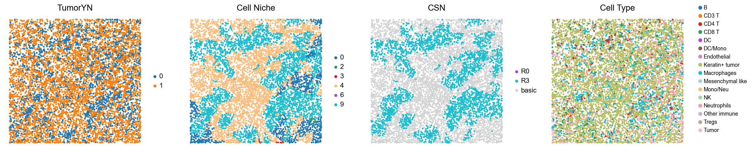
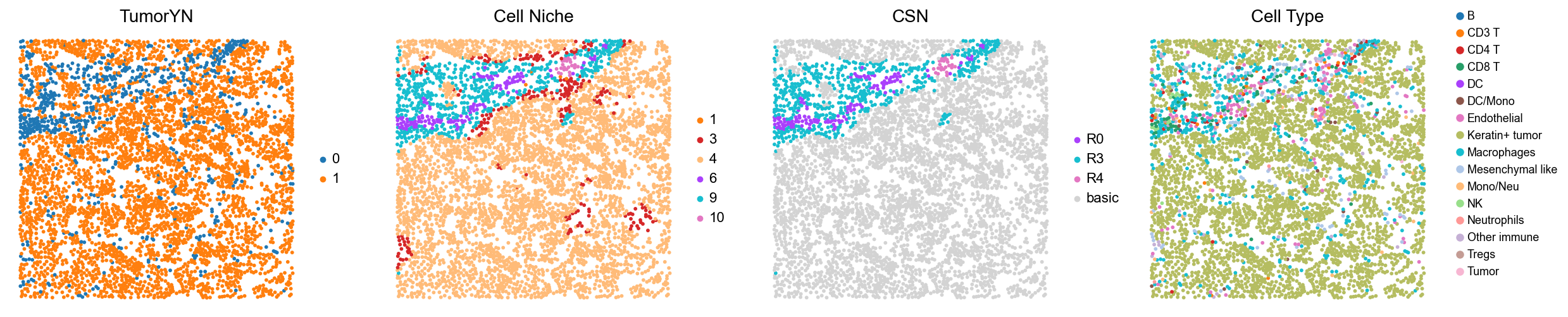
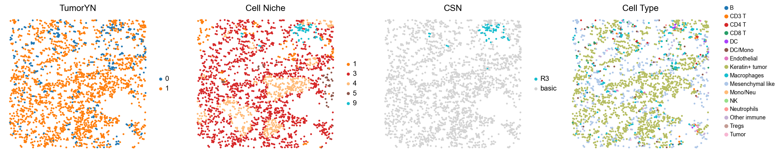
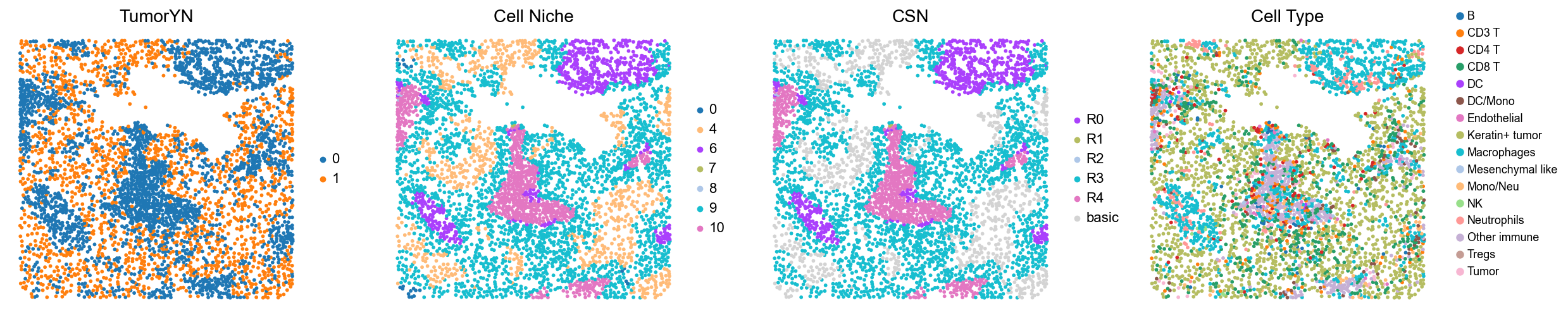
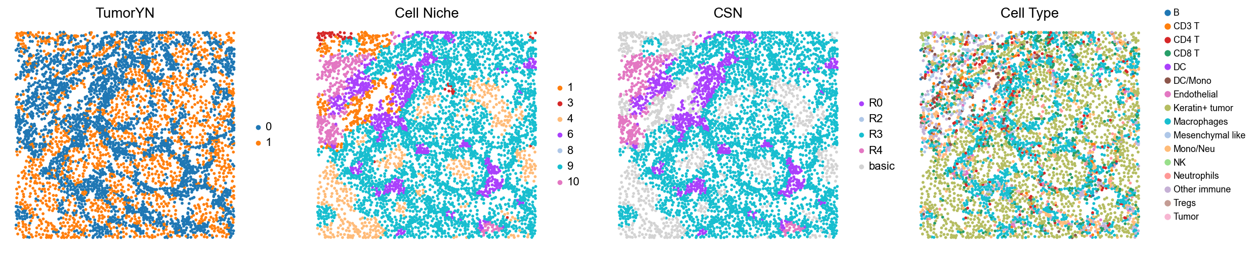
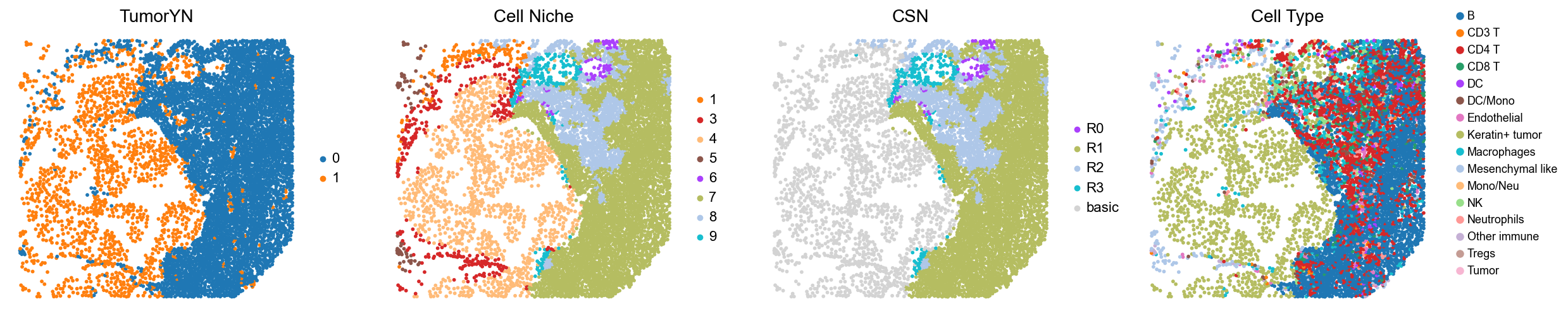
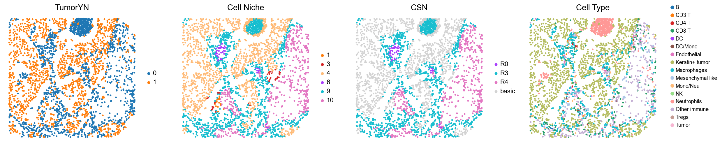
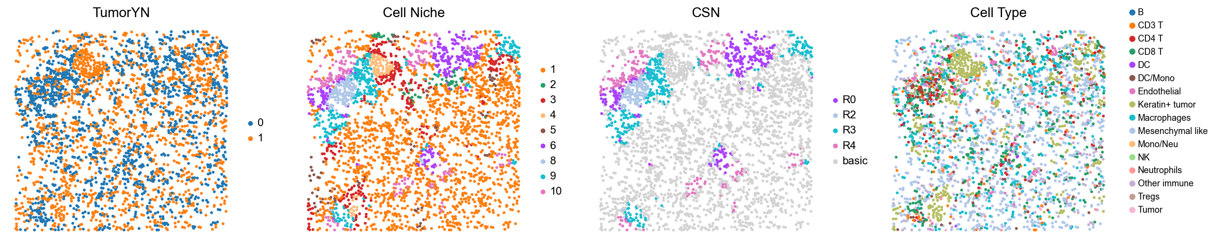
Case group (mixed group)
[18]:
for i in range(len(mixed_group)):

    print(f'p{mixed_group[i]}')
    adata = cond_concat_new[cond_concat_new.obs['slice_name'] == f'p{mixed_group[i]}', :].copy()

    fig, axes = plt.subplots(1, 4, figsize=(25, 5.5))

    sc.pl.embedding(adata, basis='spatial', color='tumorYN', palette=tumor_color_dict,
                    ax=axes[0], s=70, show=False, frameon=False, title='TumorYN', legend_fontsize=16)
    axes[0].set_title('TumorYN', fontsize=20)

    sc.pl.embedding(adata, basis='spatial', color='niche_label', palette=niche_color_dict,
                    ax=axes[1], s=70, show=False, frameon=False, title='Cell Niche', legend_fontsize=16)
    axes[1].set_title('Cell Niche', fontsize=20)

    sc.pl.embedding(adata, basis='spatial', color='csn_label', palette=csn_color_dict,
                    ax=axes[2], s=70, show=False, frameon=False, title='CSN', legend_fontsize=16)
    axes[2].set_title('CSN', fontsize=20)

    sc.pl.embedding(adata, basis='spatial', color='all_group_name', palette=ct_color_dict,
                    ax=axes[3], s=70, show=False, frameon=False, title='Cell Type', legend_fontsize=16)
    axes[3].set_title('Cell Type', fontsize=20)

    ct_legend_elements = [
        Line2D([0], [0], marker='o', color='w', label=label,
            markerfacecolor=color, markersize=10)
        for label, color in ct_color_dict.items()
    ]
    axes[3].legend(handles=ct_legend_elements, loc=(1.05, 0.1), frameon=False, ncol=1)
    axes[3].axis('off')

    plt.tight_layout()
    plt.show()
p1
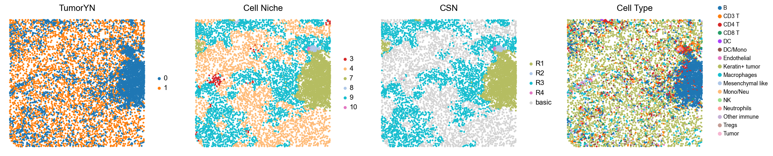
p2
p7
p8
p11
p12
p13
p14
p17
p18
p20
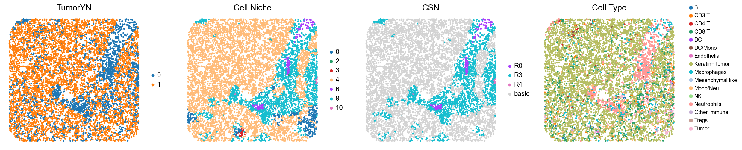
p21
p23
p27
p29
p31
p33
p38
p39
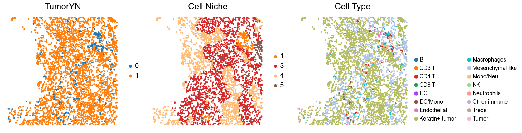
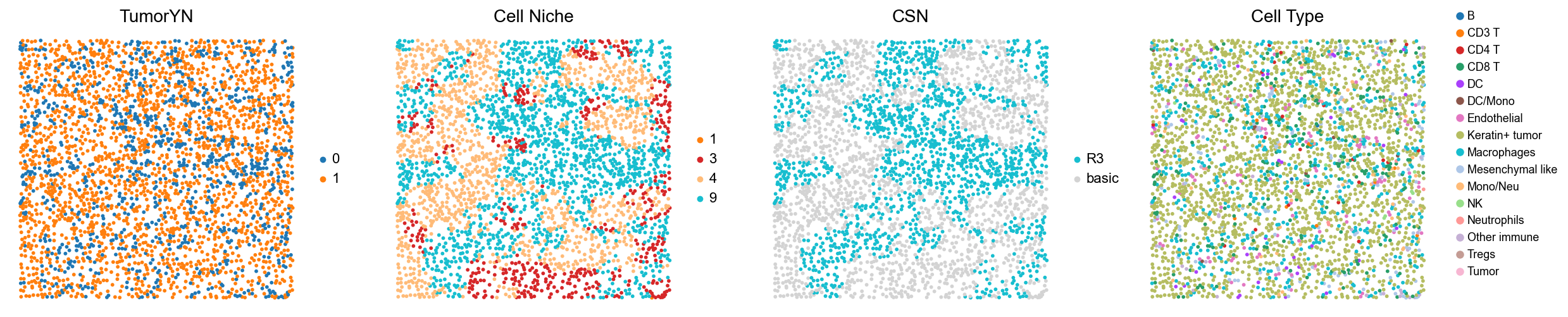
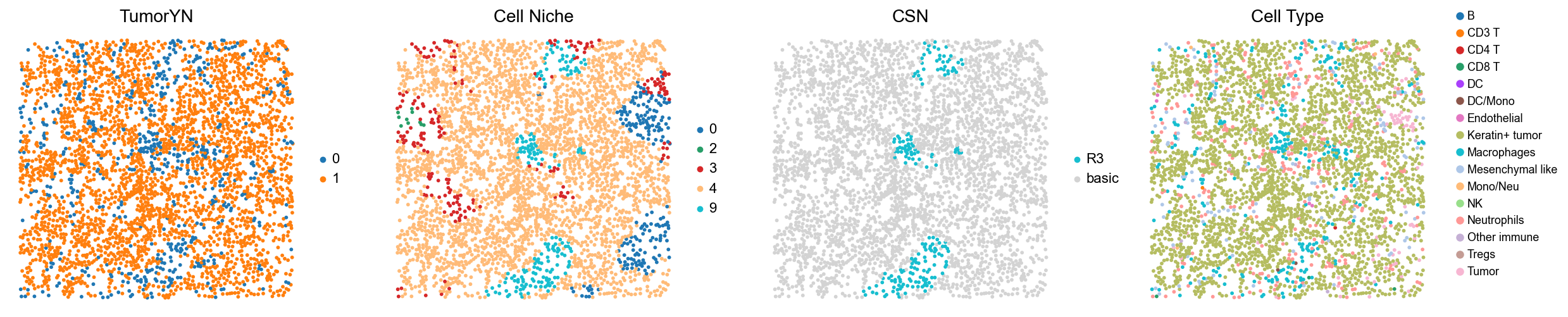
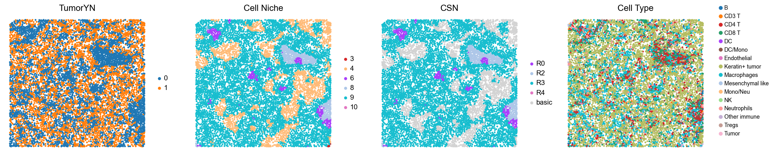
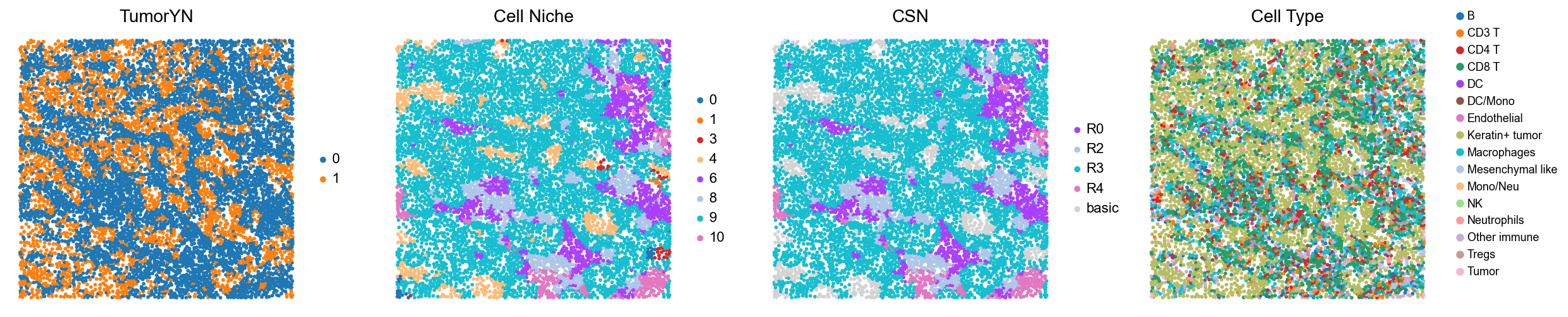
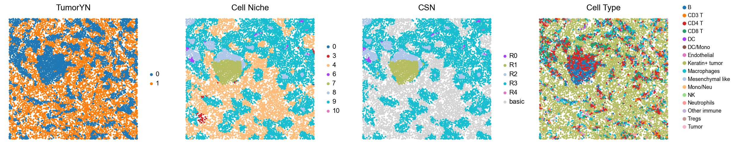
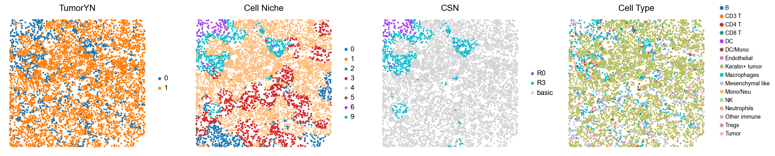
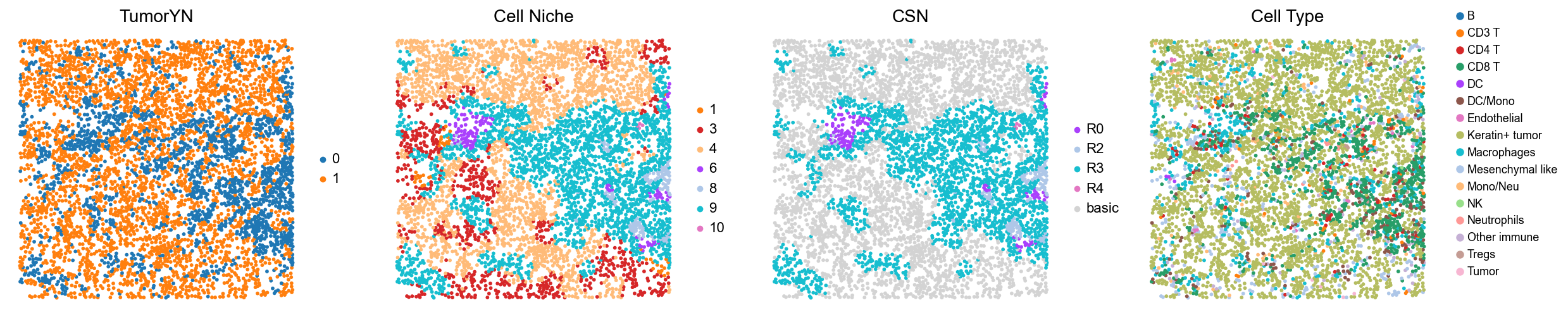
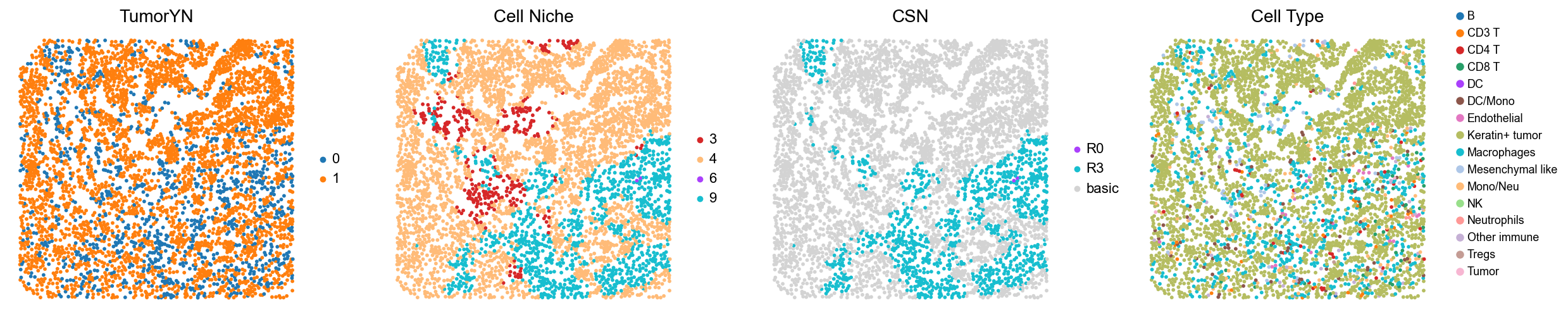
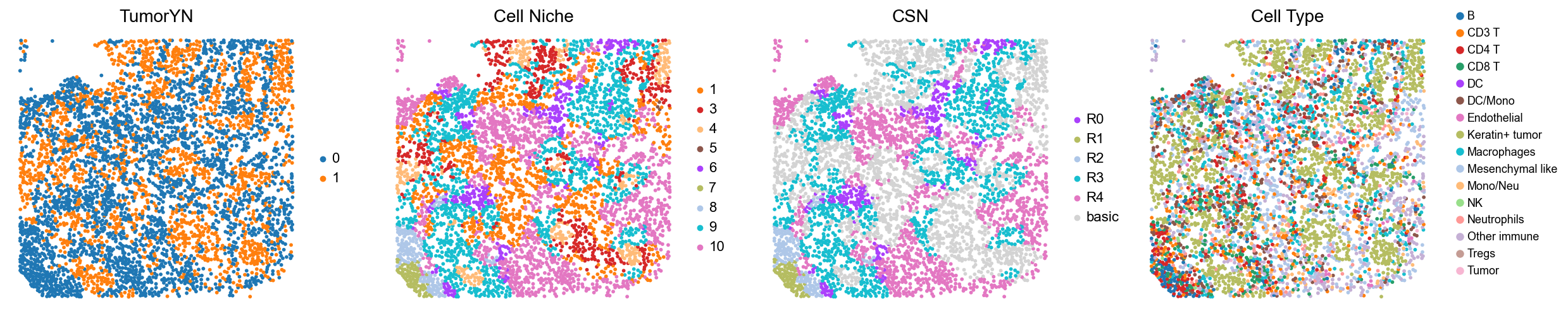
Case group (compartmentalized group)
[ ]:
for i in range(len(compartmentalized_group)):

    print(f'p{compartmentalized_group[i]}')
    adata = cond_concat_new[cond_concat_new.obs['slice_name'] == f'p{compartmentalized_group[i]}', :].copy()

    fig, axes = plt.subplots(1, 4, figsize=(25, 5.5))

    sc.pl.embedding(adata, basis='spatial', color='tumorYN', palette=tumor_color_dict,
                    ax=axes[0], s=70, show=False, frameon=False, title='TumorYN', legend_fontsize=16)
    axes[0].set_title('TumorYN', fontsize=20)

    sc.pl.embedding(adata, basis='spatial', color='niche_label', palette=niche_color_dict,
                    ax=axes[1], s=70, show=False, frameon=False, title='Cell Niche', legend_fontsize=16)
    axes[1].set_title('Cell Niche', fontsize=20)

    sc.pl.embedding(adata, basis='spatial', color='csn_label', palette=csn_color_dict,
                    ax=axes[2], s=70, show=False, frameon=False, title='CSN', legend_fontsize=16)
    axes[2].set_title('CSN', fontsize=20)

    sc.pl.embedding(adata, basis='spatial', color='all_group_name', palette=ct_color_dict,
                    ax=axes[3], s=70, show=False, frameon=False, title='Cell Type', legend_fontsize=16)
    axes[3].set_title('Cell Type', fontsize=20)

    ct_legend_elements = [
        Line2D([0], [0], marker='o', color='w', label=label,
            markerfacecolor=color, markersize=10)
        for label, color in ct_color_dict.items()
    ]
    axes[3].legend(handles=ct_legend_elements, loc=(1.05, 0.1), frameon=False, ncol=1)
    axes[3].axis('off')

    plt.tight_layout()
    plt.show()
p3
p4
p5
p6
p9
p10
p16
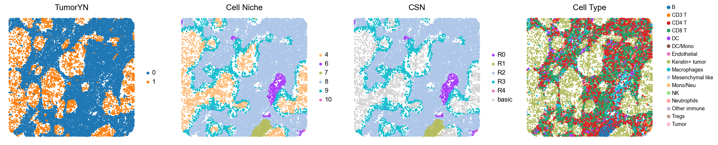
p28
p32
p34
p35
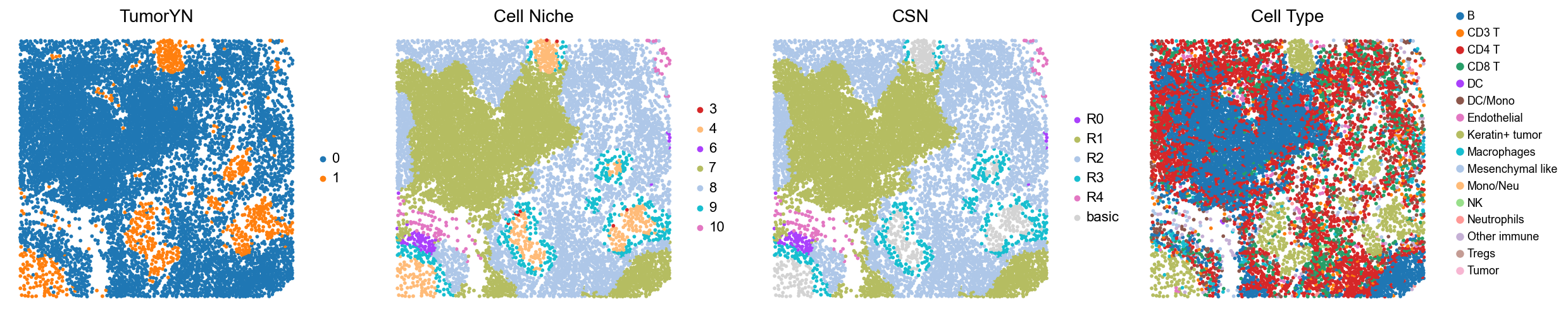
p36
p37
p40
p41
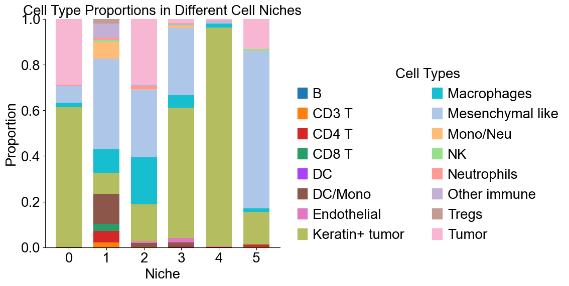
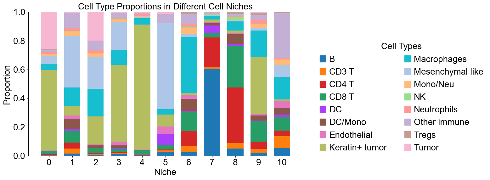
Cell type composition (control group)
[20]:
basic_niche_labels = adata_concat_new.uns['niche_label_summary'].copy()
ct_labels = sorted(cond_concat_new.obs['all_group_name'].unique())
basic_niche_dist = adata_concat_new.uns['niche_dist'].toarray().copy()
basic_cell_count_niche = adata_concat_new.uns['niche_cell_count'].copy()

fig, ax = plt.subplots(figsize=(6, 6))
bar_width = 0.7
n_niches, n_cell_types = basic_niche_dist.shape

x = np.arange(n_niches)

for j in range(n_cell_types):
    bottom = np.sum(basic_niche_dist[:, :j], axis=1)
    ax.bar(x,
           basic_niche_dist[:, j],
           bottom=bottom,
           width=bar_width,
           color=ct_color_dict[ct_labels[j]],
           label=ct_labels[j])

ax.set_ylabel('Proportion', fontsize=20)
ax.set_xlabel('Niche', fontsize=20)
ax.set_xticks(x)
ax.set_xticklabels(basic_niche_labels, rotation=0, ha='center')
ax.tick_params(axis='x', labelsize=20)
ax.tick_params(axis='y', labelsize=20)
ax.spines['top'].set_visible(False)
ax.spines['right'].set_visible(False)
ax.grid(False)

handles = [
    mpatches.Patch(color=color, label=ct)
    for ct, color in zip(celltypes, ct_colors)
]

ax.legend(handles=handles, title='Cell Types', loc=(1.05, 0.0), frameon=False, handleheight=0.8,
          handlelength=0.7, ncol=2, fontsize=20, title_fontsize=20)

plt.title('Cell Type Proportions in Different Cell Niches', fontsize=20)
plt.tight_layout()
plt.show()
Cell type composition (case group)
[21]:
cond_niche_labels = cond_concat_new.uns['niche_label_summary'].copy()
ct_labels = sorted(cond_concat_new.obs['all_group_name'].unique())
cond_niche_dist = cond_concat_new.uns['niche_dist'].toarray().copy()
cond_cell_count_niche = cond_concat_new.uns['niche_cell_count'].copy()

fig, ax = plt.subplots(figsize=(16, 6))
bar_width = 0.7
n_niches, n_cell_types = cond_niche_dist.shape

x = np.arange(n_niches)

for j in range(n_cell_types):
    bottom = np.sum(cond_niche_dist[:, :j], axis=1)
    ax.bar(x,
           cond_niche_dist[:, j],
           bottom=bottom,
           width=bar_width,
           color=ct_color_dict[ct_labels[j]],
           label=ct_labels[j])

ax.set_ylabel('Proportion', fontsize=20)
ax.set_xlabel('Niche', fontsize=20)
ax.set_xticks(x)
ax.set_xticklabels(cond_niche_labels, rotation=0, ha='center')
ax.tick_params(axis='x', labelsize=20)
ax.tick_params(axis='y', labelsize=20)
ax.spines['top'].set_visible(False)
ax.spines['right'].set_visible(False)
ax.grid(False)

handles = [
    mpatches.Patch(color=color, label=ct)
    for ct, color in zip(celltypes, ct_colors)
]

ax.legend(handles=handles, title='Cell Types', loc=(1.05, 0.0), frameon=False, handleheight=0.8,
          handlelength=0.7, ncol=2, fontsize=20, title_fontsize=20)

plt.title('Cell Type Proportions in Different Cell Niches', fontsize=20)
plt.tight_layout()
plt.show()
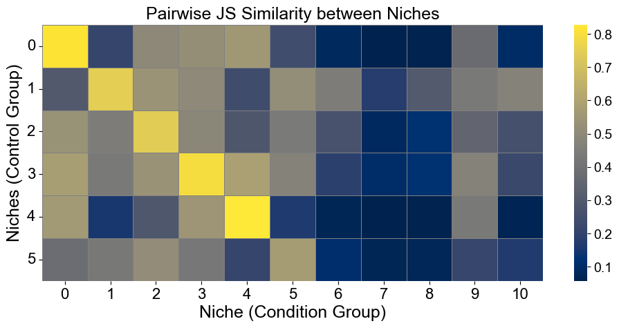
Calculate the similarity between niches from different groups
Similarities are measured using 1-JSD score
[22]:
from scipy.spatial.distance import jensenshannon
from scipy.stats import pearsonr
from sklearn.metrics.pairwise import cosine_similarity

basic_niche_dist = adata_concat_new.uns['niche_dist'].toarray().copy()
cond_niche_dist = cond_concat_new.uns['niche_dist'].toarray().copy()

basic_niche_labels = adata_concat_new.uns['niche_label_summary'].copy()
cond_niche_labels = cond_concat_new.uns['niche_label_summary'].copy()

n_niche_basic = basic_niche_dist.shape[0]
n_niche_cond = cond_niche_dist.shape[0]

js_sim = np.zeros((n_niche_basic, n_niche_cond))
# cos_sim = cosine_similarity(basic_niche_dist, cond_niche_dist)
# corr_sim = np.zeros((n_niche_basic, n_niche_cond))

for i in range(n_niche_basic):
    for j in range(n_niche_cond):
        js_sim[i, j] = 1 - jensenshannon(basic_niche_dist[i], cond_niche_dist[j], base=2)
        # corr_sim[i, j], _ = pearsonr(basic_niche_dist[i], cond_niche_dist[j])

plt.figure(figsize=(10, 5))
sns.heatmap(
    js_sim,
    cmap='cividis',
    xticklabels=cond_niche_labels,
    yticklabels=basic_niche_labels,
    linewidths=0.5,
    linecolor='gray',
)
plt.xlabel("Niche (Condition Group)", fontsize=18)
plt.ylabel("Niches (Control Group)", fontsize=18)
plt.title("Pairwise JS Similarity between Niches", fontsize=18)
plt.xticks(fontsize=16, rotation=0)
plt.yticks(fontsize=16, rotation=0)
plt.grid(False)
plt.tight_layout()
plt.show()
Cell type enrichment analysis
[23]:
ct_df = ct_enrichment_test(cond_concat_new.uns['niche_dist'],
                           cond_concat_new.uns['niche_cell_count'],
                           cond_concat_new.uns['idx2ct'],
                           cond_concat_new.uns['niche_label_summary'],
                           method='fisher',
                           alpha=0.05,
                           fdr_method='fdr_by',
                           log2fc_threshold=1,
                           prop_threshold=0.01,
                           verbose=True,
                           )
ct_df.head()
11 niches and 16 cell types in total.
[23]:
| niche_idx | niche | celltype_idx | celltype | oddsratio | p-value | q-value | log2fc | prop | enrichment | |
|---|---|---|---|---|---|---|---|---|---|---|
| 0 | 0 | 0 | 0 | B | 0.016995 | 1.395216e-90 | 2.715560e-89 | -5.800202 | 0.000967 | False |
| 1 | 0 | 0 | 1 | CD3 T | 0.221063 | 3.362091e-19 | 3.402754e-18 | -2.151897 | 0.005076 | False |
| 2 | 0 | 0 | 2 | CD4 T | 0.046033 | 4.525761e-110 | 9.957605e-109 | -4.336657 | 0.003626 | False |
| 3 | 0 | 0 | 3 | CD8 T | 0.218917 | 2.397240e-75 | 4.043723e-74 | -2.083698 | 0.021755 | False |
| 4 | 0 | 0 | 4 | DC | 0.000000 | 1.839345e-13 | 1.632975e-12 | -26.131647 | 0.000000 | False |
[24]:
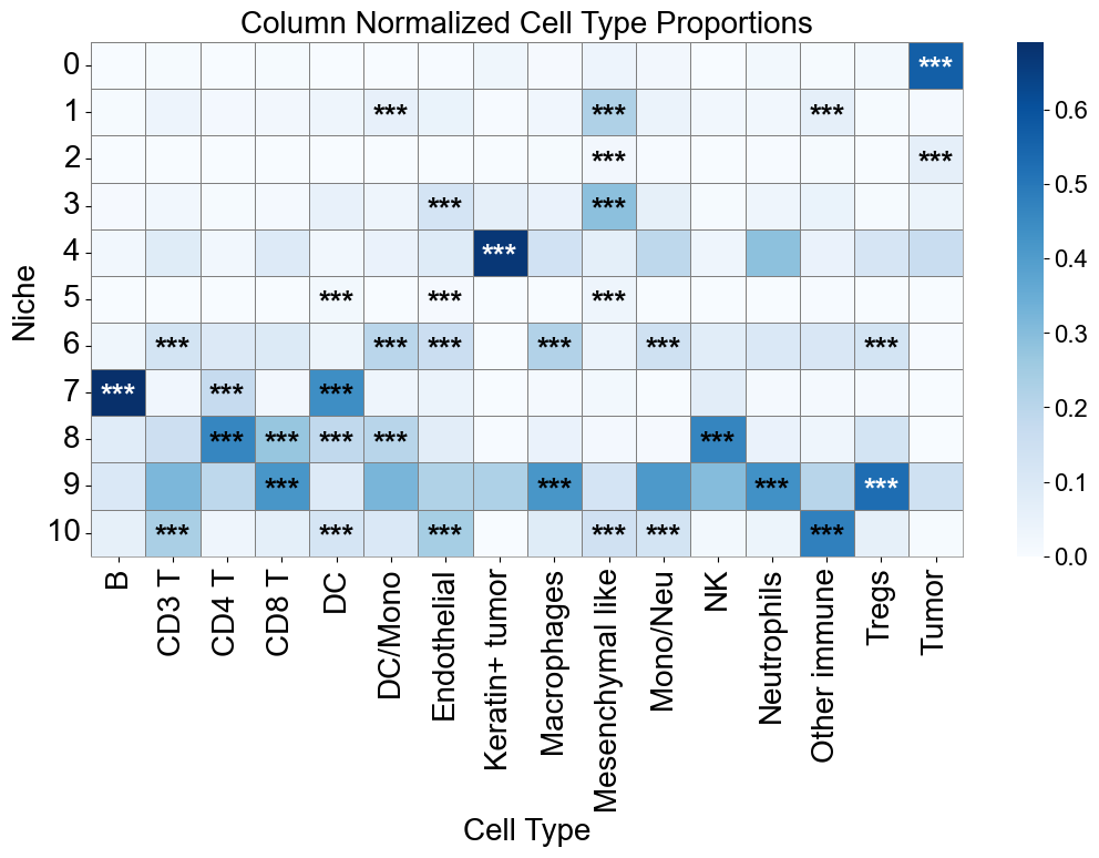
niche_labels = cond_concat_new.uns['niche_label_summary'].copy()
ct_labels = sorted(cond_concat_new.obs['all_group_name'].unique())

matrix_df = pd.DataFrame(
    data=cond_concat_new.uns['niche_dist'].toarray(),
    index=niche_labels,
    columns=ct_labels,
)

cn_dist_count = cond_concat_new.uns['niche_dist'].toarray() * cond_concat_new.uns['niche_cell_count'][:, np.newaxis]
cn_dist_norm = cn_dist_count / np.sum(cn_dist_count, axis=0)
matrix_df_norm = pd.DataFrame(
    data=cn_dist_norm,
    index=niche_labels,
    columns=ct_labels,
)

ct_df['stars'] = ct_df['q-value'].apply(p2stars)

stars_df = pd.DataFrame(
    '',
    index=matrix_df.index,
    columns=matrix_df.columns
)

for _, row in ct_df[ct_df['enrichment']].iterrows():
    niche = row['niche']
    ct    = row['celltype']
    if (niche in stars_df.index) and (ct in stars_df.columns):
        stars_df.loc[niche, ct] = row['stars']


fig, axes = plt.subplots(1, 1, figsize=(11, 8))

sns_heatmap_0 = sns.heatmap(
    matrix_df,
    cmap='Blues',
    # cbar_kws={'label': 'Cell type proportion'},
    linewidths=0.5,
    linecolor='gray',
    # square=True,
    ax=axes
)

for i, niche in enumerate(matrix_df.index):
    for j, ct in enumerate(matrix_df.columns):
        star = stars_df.iloc[i, j]
        if star:
            if matrix_df.iloc[i, j] > np.max(matrix_df.values) * 0.7:
                color='white'
            else:
                color='black'
            axes.text(j + 0.5, i + 0.6, star, ha='center', va='center', color=color, fontsize=20, fontweight='bold')

n_rows, n_cols = matrix_df.shape
axes.plot([0, n_cols], [n_rows, n_rows], color='gray', linewidth=0.5, clip_on=False)
axes.plot([n_cols, n_cols], [0, n_rows], color='gray', linewidth=0.5, clip_on=False)

axes.set_xticklabels(axes.get_xticklabels(), rotation=90, ha='center', fontsize=20)
axes.set_yticklabels(axes.get_yticklabels(), rotation=0, ha='right', fontsize=20)
axes.set_ylabel('Niche', fontsize=20)
axes.set_xlabel('Cell Type', fontsize=20)
axes.set_title('Cell Type Proportions', fontsize=20)
axes.collections[0].colorbar.ax.yaxis.label.set_size(20)
axes.collections[0].colorbar.ax.tick_params(labelsize=16)
axes.grid(False)

plt.tight_layout()
plt.show()

fig, axes = plt.subplots(1, 1, figsize=(11, 8))

sns_heatmap_1 = sns.heatmap(
    matrix_df_norm,
    cmap='Blues',
    # cbar_kws={'label': 'Cell type proportion'},
    linewidths=0.5,
    linecolor='gray',
    # square=True,
    ax=axes
)

for i, niche in enumerate(matrix_df.index):
    for j, ct in enumerate(matrix_df.columns):
        star = stars_df.iloc[i, j]
        if star:
            if matrix_df_norm.iloc[i, j] > np.max(matrix_df_norm.values) * 0.7:
                color='white'
            else:
                color='black'
            axes.text(j + 0.5, i + 0.6, star, ha='center', va='center', color=color, fontsize=20, fontweight='bold')

n_rows, n_cols = matrix_df.shape
axes.plot([0, n_cols], [n_rows, n_rows], color='gray', linewidth=0.5, clip_on=False)
axes.plot([n_cols, n_cols], [0, n_rows], color='gray', linewidth=0.5, clip_on=False)

axes.set_xticklabels(axes.get_xticklabels(), rotation=90, ha='center', fontsize=20)
axes.set_yticklabels(axes.get_yticklabels(), rotation=0, ha='right', fontsize=20)
axes.set_ylabel('Niche', fontsize=20)
axes.set_xlabel('Cell Type', fontsize=20)
axes.set_title('Column Normalized Cell Type Proportions', fontsize=20)
axes.collections[0].colorbar.ax.yaxis.label.set_size(20)
axes.collections[0].colorbar.ax.tick_params(labelsize=16)
axes.grid(False)

plt.tight_layout()
plt.show()
Immunoregulatory protein in different niches
[25]:
immunoregulatory_markers = ['PD1', 'PD-L1', 'Lag3', 'IDO']
csn_label = ['basic', 'R0', 'R1', 'R2', 'R3', 'R4']

exp_dict = {marker: {niche: {'pos': None, 'pos_tumor': None, 'pos_immune': None} for niche in csn_label} for marker in immunoregulatory_markers}

for j, niche in enumerate(csn_label):
    adata_sub = cond_concat_new[cond_concat_new.obs['csn_label'] == niche, :].copy()
    for k, marker in enumerate(immunoregulatory_markers):
        x = adata_sub[:, marker].X
        pos = (np.asarray(x).ravel() > 0.5)
        tumor = (adata_sub.obs['tumorYN'].values == '1')
        immune = ~tumor
        exp_dict[marker][niche]['pos'] = pos.mean()
        exp_dict[marker][niche]['pos_tumor'] = (pos & tumor).mean()
        exp_dict[marker][niche]['pos_immune'] = (pos & immune).mean()

records = []
for marker in immunoregulatory_markers:
    for niche in csn_label:
        records.append({'marker': marker,
                        'niche': niche,
                        'positive_fraction': exp_dict[marker][niche]['pos'],
                        'positive_fraction_tumor': exp_dict[marker][niche]['pos_tumor'],
                        'positive_fraction_immune': exp_dict[marker][niche]['pos_immune'],
                        })
df_plot = pd.DataFrame(records)
df_plot.head()
[25]:
| marker | niche | positive_fraction | positive_fraction_tumor | positive_fraction_immune | |
|---|---|---|---|---|---|
| 0 | PD1 | basic | 0.016459 | 0.007176 | 0.009283 |
| 1 | PD1 | R0 | 0.070915 | 0.000270 | 0.070645 |
| 2 | PD1 | R1 | 0.120535 | 0.000770 | 0.119765 |
| 3 | PD1 | R2 | 0.076131 | 0.000404 | 0.075727 |
| 4 | PD1 | R3 | 0.068528 | 0.007941 | 0.060587 |
[26]:
fig, axes = plt.subplots(1, 4, figsize=(14, 3), sharey=True)

for i, marker in enumerate(immunoregulatory_markers):
    df_m = df_plot[df_plot['marker'] == marker].copy()
    ax = axes[i]

    x = np.arange(len(df_m['niche']))
    width = 0.7

    ax.bar(x, df_m['positive_fraction_immune'], width, label='Immune', color="#92B4EA")
    ax.bar(x, df_m['positive_fraction_tumor'], width, bottom=df_m['positive_fraction_immune'], label='Tumor', color="#EB9E71" )
    ax.set_xticks(x)
    ax.set_xticklabels(df_m['niche'], fontsize=16)
    ax.set_ylabel(f'{marker}+ cell fraction', fontsize=16)
    ax.set_title(marker, fontsize=16)
    ax.spines['top'].set_visible(False)
    ax.spines['right'].set_visible(False)
    ax.grid(False)

handles, labels = axes[-1].get_legend_handles_labels()
fig.legend(handles, labels, bbox_to_anchor=(1.02, 0.8), ncol=1, frameon=False, fontsize=16)

plt.tight_layout(rect=[0, 0, 0.95, 1])
plt.show()
[27]:
fig, axes = plt.subplots(1, 4, figsize=(15.5, 3))

for i, marker in enumerate(immunoregulatory_markers):
    df_m = df_plot[df_plot['marker'] == marker].copy()
    ax = axes[i]

    x = np.arange(len(df_m['niche']))
    width = 0.7

    ax.bar(x, df_m['positive_fraction_immune'], width, label='Immune', color="#92B4EA")
    ax.bar(x, df_m['positive_fraction_tumor'], width, bottom=df_m['positive_fraction_immune'], label='Tumor', color="#EB9E71" )
    ax.set_xticks(x)
    ax.set_xticklabels(df_m['niche'], fontsize=16)
    ax.set_ylabel(f'{marker}+ cell fraction', fontsize=16)
    ax.set_title(marker, fontsize=16)
    ax.spines['top'].set_visible(False)
    ax.spines['right'].set_visible(False)
    ax.grid(False)

handles, labels = axes[-1].get_legend_handles_labels()
fig.legend(handles, labels, bbox_to_anchor=(1.02, 0.8), ncol=1, frameon=False, fontsize=16)

plt.tight_layout(rect=[0, 0, 0.95, 1])
plt.show()
Differential expression
In this section, we identify differential expression pattern of the same cell type across different niches.
Tumor cell from different niches
Compare Keratin+ tumor cell in the tumor-immune interaction niche (niche R3) to those in basic cell niches
Compute the mean expression of selected markers for a given cell type within one niche and in other niches across slices, then compare them using Wilcoxon tests and visualizes differences with violin plots and paired sample lines.
[28]:
from scipy.stats import wilcoxon, mannwhitneyu
from statannotations.Annotator import Annotator
np.random.seed(1234)

noi = 'R3'
ctoi = ['Keratin+ tumor']
min_cells = 20
markers = cond_concat_new.var_names.tolist()
markers = ['HLA-DR', 'HLA_Class_1', 'Vimentin', 'SMA']
n_markers = len(markers)

avg_expr_noi = [[] for _ in range(n_markers)]
avg_expr_basic = [[] for _ in range(n_markers)]
new_marker_list = []

for i, slice_name in enumerate(cond_name_list):
    adata = cond_concat_new[cond_concat_new.obs['slice_name'] == slice_name, :].copy()
    adata_noi = adata[(adata.obs['all_group_name'].isin(ctoi)) & (adata.obs['csn_label'] == noi), :].copy()
    adata_basic = adata[(adata.obs['all_group_name'].isin(ctoi)) & (adata.obs['csn_label'] == 'basic'), :].copy()
    n_cell_noi = adata_noi.shape[0]
    n_cell_basic = adata_basic.shape[0]
    if min(n_cell_noi, n_cell_basic) < min_cells:
        print(f"Skip {slice_name} due to rare cell count ({n_cell_noi} vs {n_cell_basic}).")
        continue
    for j, marker in enumerate(markers):
        avg_expr_noi[j].append(np.mean(adata_noi[:, marker].X))
        avg_expr_basic[j].append(np.mean(adata_basic[:, marker].X))

res = []
for j, marker in enumerate(markers):
    x1 = np.array(avg_expr_noi[j], dtype=float)
    x2 = np.array(avg_expr_basic[j], dtype=float)
    u, p = wilcoxon(x1, x2, alternative="two-sided")
    res.append({"marker": marker, "pvalue": p, "U": u, "n1": len(x1), "n2": len(x2)})
res_df = pd.DataFrame(res)
alpha = 0.05
sig_df = res_df[res_df["pvalue"] < alpha]#.sort_values("pvalue")
print(f"Significant markers: {sig_df.shape[0]} / {len(markers)}")
sig_markers = sig_df["marker"].tolist()

if len(sig_markers) == 0:
    print("No significant markers under the chosen threshold.")
else:
    n_plot = len(sig_markers)
    if n_plot > 5:
        ncol = 5
    else:
        ncol = n_plot
    nrow = int(np.ceil(n_plot / ncol))

    fig, axes = plt.subplots(nrow, ncol, figsize=(3.2*ncol, 4*nrow))
    axes = np.array(axes).flatten()

    for k, marker in enumerate(sig_markers):
        j = markers.index(marker)
        vals_noi = avg_expr_noi[j]
        vals_basic = avg_expr_basic[j]
        ax = axes[k]

        df_plot = pd.DataFrame({
            "expr": np.concatenate([vals_noi, vals_basic]),
            "group": [f"{noi}"]*len(vals_noi) + ["Basic"]*len(vals_basic),
        })

        colors = [ct_color_dict[ctoi[0]], '#d3d3d3']
        # sns.boxplot(data=df_plot, x="group", y="expr", ax=ax, palette=colors, width=0.5, showfliers=False)
        sns.violinplot(data=df_plot, x="group", y="expr", ax=ax, palette=colors, inner='box', cut=1, width=0.8, alpha=0.8)#, scale='width')
        # sns.stripplot(data=df_plot, x="group", y="expr", ax=ax, jitter=True, size=7, alpha=0.7, color="white", edgecolor="black", linewidth=1)

        for xpos, vals in zip([0, 1],[vals_noi, vals_basic]):
            ax.hlines(np.median(vals), xpos-0.2, xpos+0.2,
                    color='white', lw=4, zorder=3)
        pairs = [(f"{noi}", "Basic")]
        annot = Annotator(ax, pairs, data=df_plot, x='group', y='expr')
        annot.configure(test='Wilcoxon', text_format='full', loc='inside', verbose=0, fontsize=16,)
        annot.apply_and_annotate()

        n = len(vals_noi)
        jitter = 0.1
        for k in range(n):
            x1 = 0 + np.random.uniform(-jitter, jitter)
            x2 = 1 + np.random.uniform(-jitter, jitter)
            y1, y2 = vals_noi[k], vals_basic[k]
            ax.plot([x1, x2], [y1, y2], color='gray', linewidth=1, alpha=0.5, zorder=1)
            ax.scatter([x1], [y1], color='white', s=30, alpha=0.8, edgecolor='black', zorder=2)
            ax.scatter([x2], [y2], color='white', s=30, alpha=0.8, edgecolor='black', zorder=2)

        # pv = sig_df.set_index("marker").loc[marker, "pvalue"]
        ax.set_xticklabels([f"{noi}", "Basic"], fontsize=16)
        ax.tick_params(axis="y", labelsize=16)
        ax.set_title(f"{marker}", fontsize=16)
        ax.set_ylabel("Mean Scaled Expression", fontsize=16)
        ax.set_xlabel("")
        ax.spines["right"].set_visible(False)
        ax.spines["top"].set_visible(False)
        ax.grid(False)

    for ax in axes[n_plot:]:
        ax.axis("off")

    plt.suptitle(f"Keratin+ tumor ({noi} vs Basic)", fontsize=20)
    plt.tight_layout()
    plt.show()
Skip p18 due to rare cell count (10 vs 5011).
Skip p31 due to rare cell count (3 vs 2892).
Significant markers: 4 / 4
Compare per-cell (flattened) scaled expression of selected markers for a given cell type in niche noi versus basic cell niches. For each marker it builds a violin plot with median lines, runs a Mann–Whitney test (annotated on the plot), and arranges the marker subplots in a grid titled with the cell type and niche.
[29]:
noi = 'R3'
ctoi = ['Keratin+ tumor']
markers = cond_concat_new.var_names.tolist()
markers = ['HLA-DR', 'HLA_Class_1', 'Vimentin', 'SMA']

n_markers = len(markers)
new_marker_list = []

adata = cond_concat_new.copy()

adata_noi = adata[(adata.obs['all_group_name'].isin(ctoi)) & (adata.obs['csn_label'] == noi), :].copy()
adata_basic = adata[(adata.obs['all_group_name'].isin(ctoi)) & (adata.obs['csn_label'] == 'basic'), :].copy()

ncol = 4
nrow = int(np.ceil(n_markers / ncol))
fig, axes = plt.subplots(nrow, ncol, figsize=(3*ncol, 4*nrow))
axes = axes.flatten()

for j, marker in enumerate(markers):
    vals_noi = adata_noi[:, marker].X.flatten()
    vals_basic = adata_basic[:, marker].X.flatten()
    ax = axes[j]

    df_plot = pd.DataFrame({
        'expr': np.concatenate([vals_noi, vals_basic]),
        'group': [noi]*len(vals_noi)
               + ['Basic']*len(vals_basic)
    })

    colors = [ct_color_dict[ctoi[0]], '#d3d3d3']
    sns.violinplot(x='group', y='expr', data=df_plot, ax=ax, palette=colors, cut=1, inner='box', alpha=0.8)#, scale='width')

    for xpos, vals in zip([0,1],[vals_noi, vals_basic]):
        ax.hlines(np.median(vals), xpos-0.2, xpos+0.2,
                  color='white', lw=4, zorder=3)

    pairs = [(noi, 'Basic')]
    annot = Annotator(ax, pairs, data=df_plot, x='group', y='expr')
    annot.configure(test='Mann-Whitney', text_format='star', loc='inside', verbose=0, fontsize=20,)
    annot.apply_and_annotate()

    ax.set_xticklabels([noi, 'Basic'], fontsize=16)
    ax.tick_params(axis='y', labelsize=16)
    ax.set_title(marker, fontsize=16)
    ax.set_ylabel('Mean Scaled Expression', fontsize=16)
    ax.set_xlabel('Niche', fontsize=16)
    ax.spines['right'].set_visible(False)
    ax.spines['top'].set_visible(False)
    ax.grid(False)

for ax in axes[n_markers:]:
    ax.axis('off')

plt.suptitle(f"{ctoi[0]} (Niche {noi} vs Basic)", fontsize=20)
plt.tight_layout()
plt.show()
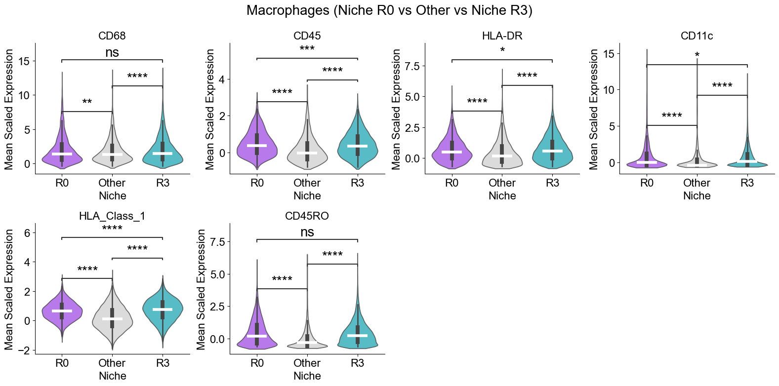
Macrophages from different niches
Compare macrophages in the two niches where they are enriched (niche R0 and R3) with macrophages in other niches.
Compute the mean expression of selected markers for a given cell type within the two niches of interest and in other niches across slices, then compare them using Wilcoxon tests and visualizes differences with violin plots and paired sample lines.
[30]:
from scipy.stats import wilcoxon

noi_list = ['R0', 'R3']
ctoi = 'Macrophages'
min_cells = 20
markers = cond_concat_new.var_names.tolist()
markers = ['CD68', 'CD45', 'HLA-DR', 'CD11c', 'HLA_Class_1', 'CD45RO']

n_markers = len(markers)

avg_expr_noi1 = [[] for _ in range(n_markers)]
avg_expr_noi2 = [[] for _ in range(n_markers)]
avg_expr_others = [[] for _ in range(n_markers)]
new_marker_list = []

for i, slice_name in enumerate(cond_name_list):

    adata = cond_concat_new[cond_concat_new.obs['slice_name'] == slice_name, :].copy()
    # adata = allconcat.copy()

    adata_noi1 = adata[(adata.obs['all_group_name'] == ctoi) & (adata.obs['csn_label'] == noi_list[0]), :].copy()
    adata_noi2 = adata[(adata.obs['all_group_name'] == ctoi) & (adata.obs['csn_label'] == noi_list[1]), :].copy()
    adata_others = adata[(adata.obs['all_group_name'] == ctoi) & ~(adata.obs['csn_label'].isin(noi_list)), :].copy()

    n_cell_noi1 = adata_noi1.shape[0]
    n_cell_noi2 = adata_noi2.shape[0]
    n_cell_others = adata_others.shape[0]

    if min(n_cell_noi1, n_cell_noi2, n_cell_others) < min_cells:
        print(f"Skip {slice_name} due to rare cell count ({n_cell_noi1} vs {n_cell_noi2} vs {n_cell_others}).")
        continue

    for j, marker in enumerate(markers):
        avg_expr_noi1[j].append(np.mean(adata_noi1[:, marker].X))
        avg_expr_noi2[j].append(np.mean(adata_noi2[:, marker].X))
        avg_expr_others[j].append(np.mean(adata_others[:, marker].X))

alpha = 0.05
pairs = [(noi_list[0], "other"), ("other", noi_list[1]), (noi_list[0], noi_list[1])]

test_res = []
for j, marker in enumerate(markers):
    vals1 = np.array(avg_expr_noi1[j], dtype=float)
    vals2 = np.array(avg_expr_others[j], dtype=float)
    vals3 = np.array(avg_expr_noi2[j], dtype=float)

    p12 = wilcoxon(vals1, vals2, alternative="two-sided").pvalue
    p23 = wilcoxon(vals2, vals3, alternative="two-sided").pvalue
    p13 = wilcoxon(vals1, vals3, alternative="two-sided").pvalue

    pvals = np.array([p12, p23, p13], dtype=float)
    any_sig = np.any(pvals < alpha)
    test_res.append({
        "marker": marker,
        "n": len(vals1),
        "p_R0_other": p12,
        "p_other_R3": p23,
        "p_R0_R3": p13,
        "p_min": float(np.min(pvals)),
        "any_sig": bool(any_sig)
    })

test_df = pd.DataFrame(test_res)
plot_markers = test_df.loc[test_df["any_sig"], "marker"].tolist()

print(f"Markers to plot: {len(plot_markers)} / {len(markers)}")


if len(plot_markers) == 0:
    print("No markers passed the significance filter. Nothing to plot.")
else:
    n_plot = len(plot_markers)
    if n_plot > 4:
        ncol = 4
    else:
        ncol = n_plot
    nrow = int(np.ceil(n_plot / ncol))
    fig, axes = plt.subplots(nrow, ncol, figsize=(4*ncol, 4*nrow))
    axes = np.array(axes).flatten()

    colors = [csn_color_dict[noi_list[0]], "lightgray", csn_color_dict[noi_list[1]]]

    for idx, marker in enumerate(plot_markers):
        j = markers.index(marker)

        vals1 = np.array(avg_expr_noi1[j], dtype=float)
        vals2 = np.array(avg_expr_others[j], dtype=float)
        vals3 = np.array(avg_expr_noi2[j], dtype=float)

        ax = axes[idx]

        df_plot = pd.DataFrame({
            "expr": np.concatenate([vals1, vals2, vals3]),
            "group": [noi_list[0]]*len(vals1) + ["other"]*len(vals2) + [noi_list[1]]*len(vals3),
        })

        sns.violinplot(x="group", y="expr", data=df_plot, ax=ax, palette=colors, cut=1, inner='box', alpha=0.8)#, scale="width")
        # sns.boxplot(data=df_plot, x="group", y="expr", ax=ax, width=0.5, palette=colors, showfliers=False)
        # sns.stripplot(data=df_plot, x="group", y="expr", ax=ax, jitter=True, size=7, alpha=0.7, color="white", edgecolor="black", linewidth=1)

        for xpos, vals in zip([0, 1, 2], [vals1, vals2, vals3]):
            ax.hlines(np.median(vals), xpos-0.2, xpos+0.2,
                      color="white", lw=4, zorder=3)
        pairs = [(noi_list[0], 'other'), ('other', noi_list[1]), (noi_list[0], noi_list[1])]
        annot = Annotator(ax, pairs, data=df_plot, x='group', y='expr')
        annot.configure(test='Wilcoxon', text_format='full', loc='inside', verbose=0, fontsize=16,)
        annot.apply_and_annotate()

        jitter = 0.1
        for k in range(len(vals1)):
            xx1 = 0 + np.random.uniform(-jitter, jitter)
            xx2 = 1 + np.random.uniform(-jitter, jitter)
            xx3 = 2 + np.random.uniform(-jitter, jitter)

            ax.plot([xx1, xx2], [vals1[k], vals2[k]], color="gray", linewidth=0.8, alpha=0.5, zorder=1)
            ax.plot([xx2, xx3], [vals2[k], vals3[k]], color="gray", linewidth=0.8, alpha=0.5, zorder=1)

            ax.scatter(xx1, vals1[k], color='white', s=30, alpha=0.8, edgecolor="black", zorder=2)
            ax.scatter(xx2, vals2[k], color='white', s=30, alpha=0.8, edgecolor="black", zorder=2)
            ax.scatter(xx3, vals3[k], color='white', s=30, alpha=0.8, edgecolor="black", zorder=2)

        row = test_df.set_index("marker").loc[marker]
        ax.set_title(f"{marker}", fontsize=16)

        ax.set_xticklabels([noi_list[0], "Other", noi_list[1]], fontsize=16)
        ax.tick_params(axis="y", labelsize=16)
        ax.set_ylabel("Mean Scaled Expression", fontsize=16)
        ax.set_xlabel("Niche", fontsize=16)
        ax.spines["top"].set_visible(False)
        ax.spines["right"].set_visible(False)
        ax.grid(False)

    for ax in axes[n_plot:]:
        ax.axis("off")

    plt.suptitle(f"{ctoi} (Niche {noi_list[0]} vs Other vs Niche {noi_list[1]})", fontsize=20)
    plt.tight_layout()
    plt.show()
Skip p1 due to rare cell count (0 vs 162 vs 119).
Skip p2 due to rare cell count (0 vs 303 vs 208).
Skip p7 due to rare cell count (0 vs 82 vs 163).
Skip p8 due to rare cell count (0 vs 22 vs 247).
Skip p11 due to rare cell count (1 vs 355 vs 218).
Skip p17 due to rare cell count (10 vs 432 vs 136).
Skip p18 due to rare cell count (0 vs 2 vs 310).
Skip p21 due to rare cell count (0 vs 26 vs 185).
Skip p31 due to rare cell count (0 vs 5 vs 267).
Skip p33 due to rare cell count (0 vs 17 vs 135).
Skip p35 due to rare cell count (18 vs 17 vs 129).
Skip p38 due to rare cell count (0 vs 307 vs 379).
Skip p40 due to rare cell count (0 vs 19 vs 94).
Markers to plot: 6 / 6
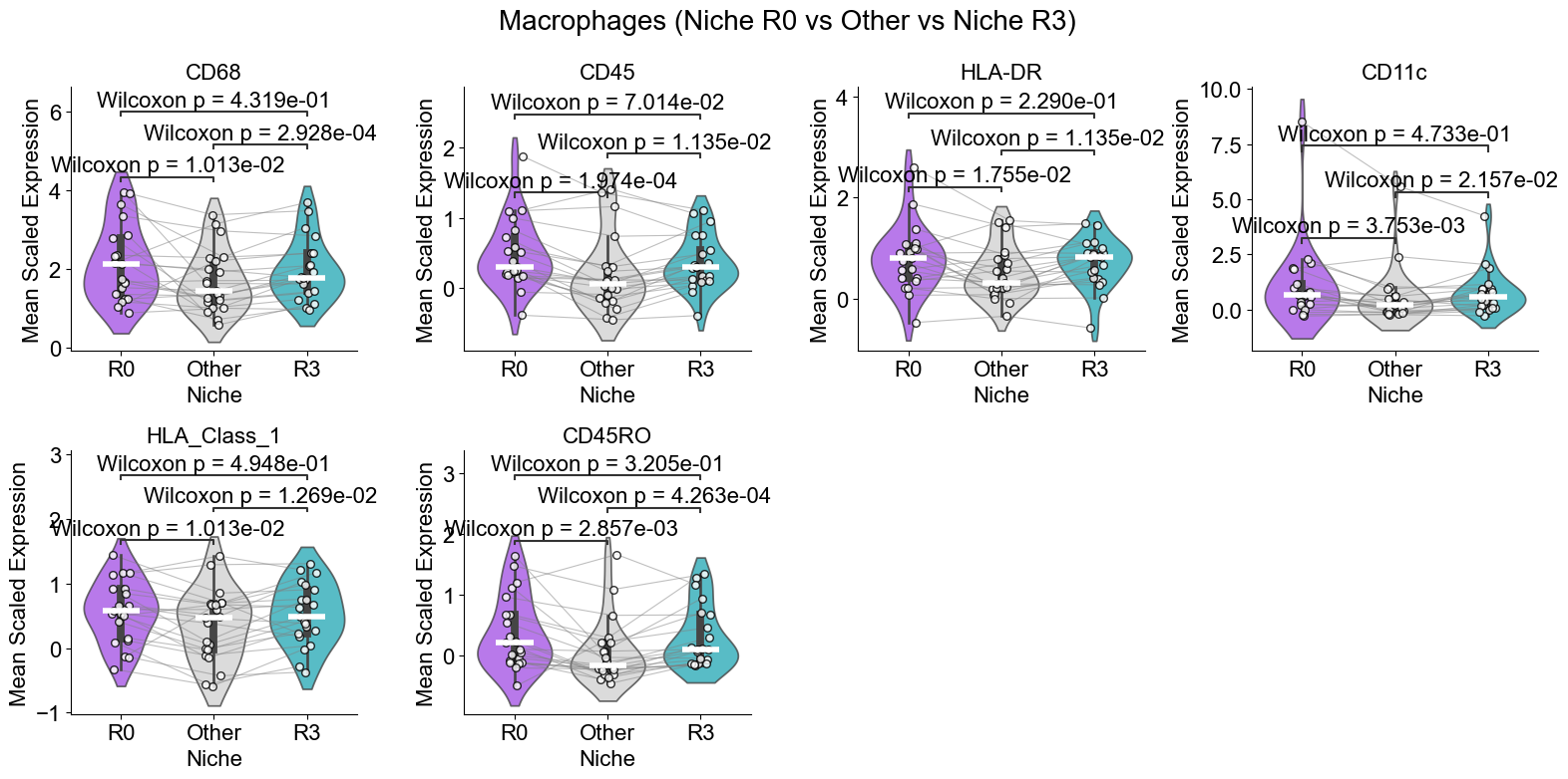
Compare per-cell (flattened) scaled expression of selected markers for a given cell type in niches in noi_list versus all other niches. For each marker it builds a violin plot with median lines, runs a Mann–Whitney test (annotated on the plot), and arranges the marker subplots in a grid titled with the cell type and niche.
[31]:
noi_list = ['R0', 'R3']
ctoi = 'Macrophages'
markers = cond_concat_new.var_names.tolist()
markers = ['CD68', 'CD45', 'HLA-DR', 'CD11c', 'HLA_Class_1', 'CD45RO']

n_markers = len(markers)
new_marker_list = []

adata = cond_concat_new.copy()

adata_noi1 = adata[(adata.obs['all_group_name'] == ctoi) & (adata.obs['csn_label'] == noi_list[0]), :].copy()
adata_noi2 = adata[(adata.obs['all_group_name'] == ctoi) & (adata.obs['csn_label'] == noi_list[1]), :].copy()
adata_other = adata[(adata.obs['all_group_name'] == ctoi) & ~(adata.obs['csn_label'].isin(noi_list)), :].copy()

ncol = 4
nrow = int(np.ceil(n_markers / ncol))
fig, axes = plt.subplots(nrow, ncol, figsize=(4*ncol, 4*nrow))
axes = axes.flatten()

for j, marker in enumerate(markers):
    vals_noi1 = adata_noi1[:, marker].X.flatten()
    vals_noi2 = adata_noi2[:, marker].X.flatten()
    vals_other = adata_other[:, marker].X.flatten()
    ax = axes[j]

    df_plot = pd.DataFrame({
        'expr': np.concatenate([vals_noi1, vals_other, vals_noi2]),
        'group': [noi_list[0]]*len(vals_noi1)
               + ['other']*len(vals_other)
               + [noi_list[1]]*len(vals_noi2)
    })

    colors = [csn_color_dict[noi_list[0]], 'lightgray', csn_color_dict[noi_list[1]]]
    sns.violinplot(x='group', y='expr', data=df_plot, ax=ax, palette=colors, cut=1, inner='box', alpha=0.8)#, scale='width')

    for xpos, vals in zip([0,1,2],[vals_noi1, vals_other, vals_noi2]):
        ax.hlines(np.median(vals), xpos-0.2, xpos+0.2,
                  color='white', lw=4, zorder=3)

    pairs = [(noi_list[0], 'other'), ('other', noi_list[1]), (noi_list[0], noi_list[1])]
    annot = Annotator(ax, pairs, data=df_plot, x='group', y='expr')
    annot.configure(test='Mann-Whitney', text_format='star', loc='inside', verbose=0, fontsize=20,)
    annot.apply_and_annotate()

    ax.set_xticklabels([noi_list[0], 'Other', noi_list[1]], fontsize=16)
    ax.tick_params(axis='y', labelsize=16)
    ax.set_title(marker, fontsize=16)
    ax.set_ylabel('Mean Scaled Expression', fontsize=16)
    ax.set_xlabel('Niche', fontsize=16)
    ax.spines['right'].set_visible(False)
    ax.spines['top'].set_visible(False)
    ax.grid(False)

for ax in axes[n_markers:]:
    ax.axis('off')

plt.suptitle(f"{ctoi} (Niche {noi_list[0]} vs Other vs Niche {noi_list[1]})", fontsize=20)
plt.tight_layout()
plt.show()
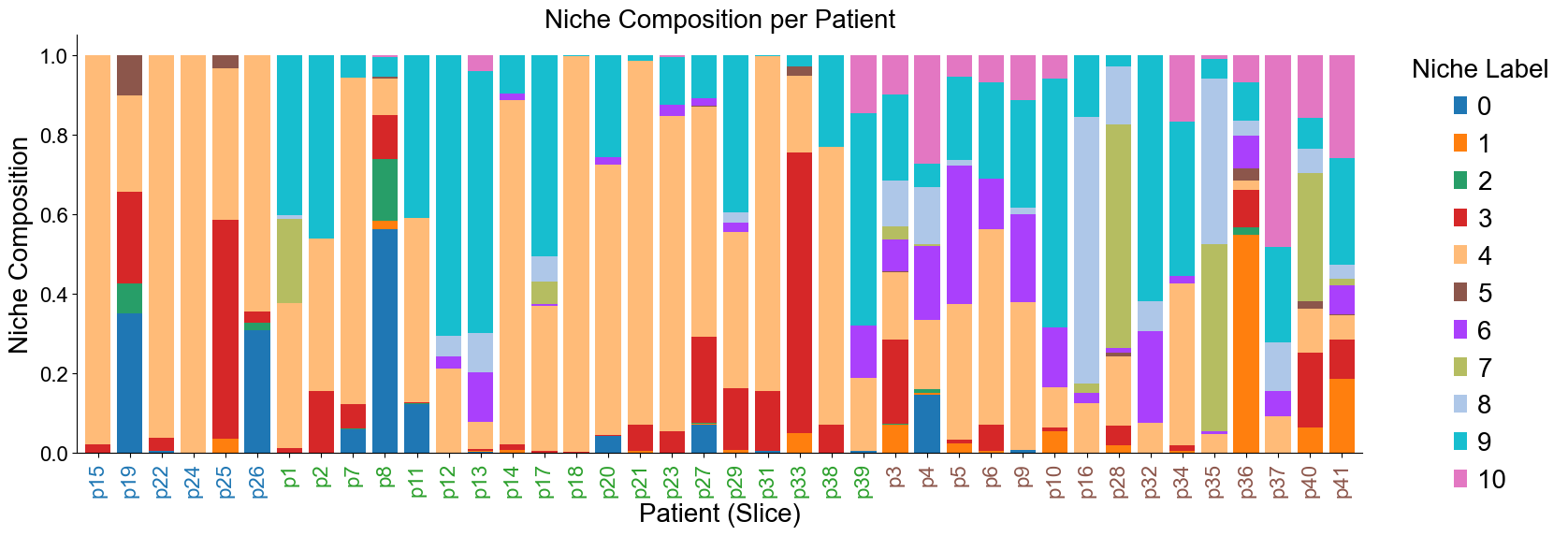
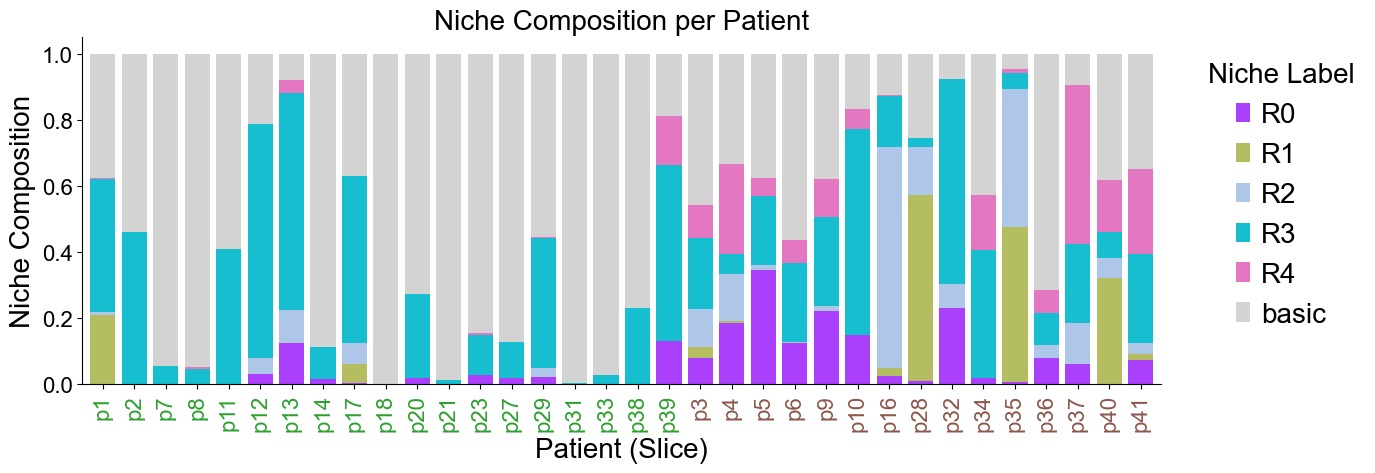
Niche composition for different patients (slices)
[32]:
from scipy.cluster.hierarchy import linkage, leaves_list

group_colors = {
    'cold': '#1f77b4',
    'mixed': '#2ca02c',
    'compartmentalized': '#8c564b'
}
slice_color_dict = {}
for i in cold_group:
    slice_color_dict[f'p{i}'] = group_colors['cold']
for i in mixed_group:
    slice_color_dict[f'p{i}'] = group_colors['mixed']
for i in compartmentalized_group:
    slice_color_dict[f'p{i}'] = group_colors['compartmentalized']
[33]:
df_list = []

df_list.append(adata_concat_new.obs[['niche_label', 'slice_name']].copy())
df_list.append(cond_concat_new.obs[['niche_label', 'slice_name']].copy())
df = pd.concat(df_list, axis=0)

comp = pd.crosstab(df['slice_name'], df['niche_label'], normalize='index').sort_index()
cond_niche_labels = cond_concat_new.uns['niche_label_summary'].copy()
comp = comp[cond_niche_labels]

# linkage_result = linkage(comp.values, metric='correlation')
# ordered_indices = leaves_list(linkage_result)
# comp = comp.iloc[ordered_indices]
comp = comp.loc[slice_color_dict.keys()]

plt.figure(figsize=(17, 6))
ax = comp.plot(
    kind='bar',
    stacked=True,
    width=0.8,
    color=niche_colors,
    ax=plt.gca()
)

plt.ylabel('Niche Composition', fontsize=20)
plt.xlabel('Patient (Slice)', fontsize=20)
plt.title('Niche Composition per Patient', fontsize=20)
plt.yticks(fontsize=16)

ax.set_xticks(range(len(comp.index)))
ax.set_xticklabels(comp.index, rotation=90, ha='center', fontsize=16)

for tick_label in ax.get_xticklabels():
    slice_name = tick_label.get_text()
    if slice_name in slice_color_dict:
        tick_label.set_color(slice_color_dict[slice_name])

ax.legend(title='Niche Label', bbox_to_anchor=(1.02, 1), loc='upper left', fontsize=20, title_fontsize=20, frameon=False)
ax.spines['top'].set_visible(False)
ax.spines['right'].set_visible(False)
plt.grid(False)
plt.tight_layout()
plt.show()
[34]:
df_list = []

# adata_concat_new.obs['csn_label'] = 'basic'
# df_list.append(adata_concat_new.obs[['csn_label', 'slice_name']].copy())
df_list.append(cond_concat_new.obs[['csn_label', 'slice_name']].copy())
df = pd.concat(df_list, axis=0)

comp = pd.crosstab(df['slice_name'], df['csn_label'], normalize='index').sort_index()
cond_niche_labels =  csns + ['basic']
comp = comp[cond_niche_labels]

# linkage_result = linkage(comp.values, method='ward', metric='euclidean')
# ordered_indices = leaves_list(linkage_result)
# comp = comp.iloc[ordered_indices]
comp = comp.loc[[slice_name for slice_name in slice_color_dict.keys() if slice_name not in ['p15', 'p19', 'p22', 'p24', 'p25', 'p26']]]

plt.figure(figsize=(14, 5))
ax = comp.plot(
    kind='bar',
    stacked=True,
    width=0.8,
    color=csn_color_dict.values(),
    ax=plt.gca()
)

plt.ylabel('Niche Composition', fontsize=20)
plt.xlabel('Patient (Slice)', fontsize=20)
plt.title('Niche Composition per Patient', fontsize=20)
plt.yticks(fontsize=16)

ax.set_xticks(range(len(comp.index)))
ax.set_xticklabels(comp.index, rotation=90, ha='center', fontsize=16)

for tick_label in ax.get_xticklabels():
    slice_name = tick_label.get_text()
    if slice_name in slice_color_dict:
        tick_label.set_color(slice_color_dict[slice_name])

ax.legend(title='Niche Label', bbox_to_anchor=(1.02, 1), loc='upper left', fontsize=20, title_fontsize=20, frameon=False)
ax.spines['top'].set_visible(False)
ax.spines['right'].set_visible(False)
plt.grid(False)
plt.tight_layout()
plt.show()
The niche composition comparison between mixed and compartmentalized group
[36]:
import plotly.express as px
import plotly.graph_objects as go
from plotly.subplots import make_subplots

# Pie chart data
mixed_slice_name = [f'p{id}' for id in mixed_group]
compart_slice_name = [f'p{id}' for id in compartmentalized_group]

mixed_adata = cond_concat_new[cond_concat_new.obs['slice_name'].isin(mixed_slice_name), :].copy()
compart_adata = cond_concat_new[cond_concat_new.obs['slice_name'].isin(compart_slice_name), :].copy()

mixed_counts = mixed_adata.obs['niche_label'].value_counts(normalize=True)
compart_counts = compart_adata.obs['niche_label'].value_counts(normalize=True)

ordered_labels_mixed = [label for label in niche_color_dict.keys() if label in mixed_counts.index]
mixed_values = [mixed_counts[label] for label in ordered_labels_mixed]
mixed_colors = [niche_color_dict[label] for label in ordered_labels_mixed]
mixed_labels_text = [f"{v*100:.1f}%" for v in mixed_values]

ordered_labels_compart = [label for label in niche_color_dict.keys() if label in compart_counts.index]
compart_values = [compart_counts[label] for label in ordered_labels_compart]
compart_colors = [niche_color_dict[label] for label in ordered_labels_compart]
compart_labels_text = [f"{v*100:.1f}%" for v in compart_values]

# Build subplots
fig = make_subplots(
    rows=1, cols=2, specs=[[{'type': 'domain'}, {'type': 'domain'}]],
    subplot_titles=("Mixed Group", "Compartmentalized Group")
)

fig.add_trace(go.Pie(
    values=mixed_values,
    labels=ordered_labels_mixed,
    name="Mixed",
    marker=dict(colors=mixed_colors,
                # line=dict(color='#FFFFFF', width=2),
                ),
    text=mixed_labels_text,
    textinfo='label+text',  # label + formatted percent
    textposition='outside',
    pull=[0.05]*len(mixed_values),
    hole=0,
    sort=True
), row=1, col=1)

fig.add_trace(go.Pie(
    values=compart_values,
    labels=ordered_labels_compart,
    name="Compartmentalized",
    marker=dict(colors=compart_colors,
                # line=dict(color='#FFFFFF', width=2),
                ),
    text=compart_labels_text,
    textinfo='label+text',
    textposition='outside',
    pull=[0.05]*len(compart_values),
    hole=0,
    sort=True
), row=1, col=2)

# Update layout
fig.update_layout(
    title_text="Niche Composition Comparison",
    title_x=0.5,
    height=700,
    width=1100,
    showlegend=False,
    margin=dict(t=100, b=50),
    font=dict(size=16)
)

fig.show()
Data type cannot be displayed: application/vnd.plotly.v1+json
The niche composition comparison between mixed and compartmentalized group (all basic cell niches labeled as “basic”)
[37]:
# Pie chart data
mixed_counts = mixed_adata.obs['csn_label'].value_counts(normalize=True)
compart_counts = compart_adata.obs['csn_label'].value_counts(normalize=True)

ordered_labels_mixed = [label for label in csn_color_dict.keys() if label in mixed_counts.index]
mixed_values = [mixed_counts[label] for label in ordered_labels_mixed]
mixed_colors = [csn_color_dict[label] for label in ordered_labels_mixed]
mixed_labels_text = [f"{v*100:.1f}%" for v in mixed_values]

ordered_labels_compart = [label for label in csn_color_dict.keys() if label in compart_counts.index]
compart_values = [compart_counts[label] for label in ordered_labels_compart]
compart_colors = [csn_color_dict[label] for label in ordered_labels_compart]
compart_labels_text = [f"{v*100:.1f}%" for v in compart_values]

# Build subplots
fig = make_subplots(
    rows=1, cols=2, specs=[[{'type': 'domain'}, {'type': 'domain'}]],
    subplot_titles=("Mixed Group", "Compartmentalized Group")
)

fig.add_trace(go.Pie(
    values=mixed_values,
    labels=ordered_labels_mixed,
    name="Mixed",
    marker=dict(colors=mixed_colors,
                # line=dict(color='#FFFFFF', width=2),
                ),
    text=mixed_labels_text,
    textinfo='label+text',  # label + formatted percent
    textposition='outside',
    pull=[0.05]*len(mixed_values),
    hole=0,
    sort=True
), row=1, col=1)

fig.add_trace(go.Pie(
    values=compart_values,
    labels=ordered_labels_compart,
    name="Compartmentalized",
    marker=dict(colors=compart_colors,
                # line=dict(color='#FFFFFF', width=2),
                ),
    text=compart_labels_text,
    textinfo='label+text',
    textposition='outside',
    pull=[0.05]*len(compart_values),
    hole=0,
    sort=True
), row=1, col=2)

# Update layout
fig.update_layout(
    title_text="Niche Composition Comparison",
    title_x=0.5,
    height=500,
    width=1100,
    showlegend=False,
    margin=dict(t=100, b=50),
    font=dict(size=16)
)

fig.show()
Data type cannot be displayed: application/vnd.plotly.v1+json
The condition-specific niche composition comparison between mixed and compartmentalized group
[38]:
# Pie chart data
mixed_adata = mixed_adata[mixed_adata.obs['csn_label'] != 'basic', :].copy()
compart_adata = compart_adata[compart_adata.obs['csn_label'] != 'basic', :].copy()

mixed_counts = mixed_adata.obs['csn_label'].value_counts(normalize=True)
compart_counts = compart_adata.obs['csn_label'].value_counts(normalize=True)

ordered_labels_mixed = [label for label in csn_color_dict.keys() if label in mixed_counts.index]
mixed_values = [mixed_counts[label] for label in ordered_labels_mixed]
mixed_colors = [csn_color_dict[label] for label in ordered_labels_mixed]
mixed_labels_text = [f"{v*100:.1f}%" for v in mixed_values]

ordered_labels_compart = [label for label in csn_color_dict.keys() if label in compart_counts.index]
compart_values = [compart_counts[label] for label in ordered_labels_compart]
compart_colors = [csn_color_dict[label] for label in ordered_labels_compart]
compart_labels_text = [f"{v*100:.1f}%" for v in compart_values]

# Build subplots
fig = make_subplots(
    rows=1, cols=2, specs=[[{'type': 'domain'}, {'type': 'domain'}]],
    subplot_titles=("Mixed Group", "Compartmentalized Group")
)

fig.add_trace(go.Pie(
    values=mixed_values,
    labels=ordered_labels_mixed,
    name="Mixed",
    marker=dict(colors=mixed_colors,
                # line=dict(color='#FFFFFF', width=2),
                ),
    text=mixed_labels_text,
    textinfo='label+text',  # label + formatted percent
    textposition='outside',
    pull=[0.05]*len(mixed_values),
    hole=0,
    sort=True
), row=1, col=1)

fig.add_trace(go.Pie(
    values=compart_values,
    labels=ordered_labels_compart,
    name="Compartmentalized",
    marker=dict(colors=compart_colors,
                # line=dict(color='#FFFFFF', width=2),
                ),
    text=compart_labels_text,
    textinfo='label+text',
    textposition='outside',
    pull=[0.05]*len(compart_values),
    hole=0,
    sort=True
), row=1, col=2)

# Update layout
fig.update_layout(
    title_text="Niche Composition Comparison",
    title_x=0.5,
    height=500,
    width=1100,
    showlegend=False,
    margin=dict(t=100, b=50),
    font=dict(size=16)
)

fig.show()
Data type cannot be displayed: application/vnd.plotly.v1+json
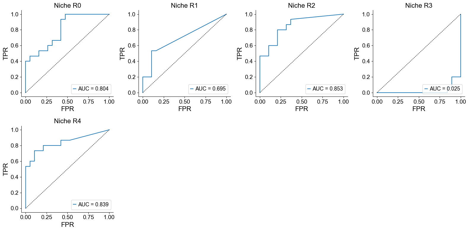
Classification of mixed and compartmentalized group using niche proportion
compartmentalized group = 1; mixed group = 0
Proportion of a specific CSN across all CSNs
[39]:
from sklearn.metrics import roc_curve, auc

group_labels = []
for cond_name in cond_name_list:
    adata = cond_concat[cond_concat.obs['slice_name'] == cond_name, :].copy()
    group = int(adata.obs['sample_types'][0] == 'compartmentalized')
    group_labels.append(group)

group_labels = np.array(group_labels)

ncol = 4
nrow = int(np.ceil((len(csns)) / ncol))
fig, axes = plt.subplots(nrow, ncol, figsize=(4*ncol, 4*nrow))
axes = axes.flatten()

for i, roi in enumerate(csns):

    ratios = []
    for cond_name in cond_name_list:
        adata = cond_concat[cond_concat.obs['slice_name'] == cond_name, :].copy()
        roi_ratio = (adata.obs['csn_label'] == roi).mean() / (1 - (adata.obs['csn_label'] == 'basic').mean())
        ratios.append(roi_ratio)

    ratios = np.array(ratios)

    # ROC curve
    fpr, tpr, _ = roc_curve(group_labels, ratios)
    roc_auc = auc(fpr, tpr)

    ax = axes[i]
    ax.plot(fpr, tpr, label=f'AUC = {roc_auc:.3f}')
    ax.plot([0, 1], [0, 1], 'k--', linewidth=0.8)
    ax.set_title(f'Niche {roi}', fontsize=16)
    ax.set_xlabel('FPR', fontsize=16)
    ax.set_ylabel('TPR', fontsize=16)
    ax.grid(False)
    ax.spines['top'].set_visible(False)
    ax.spines['right'].set_visible(False)
    ax.legend(loc='lower right')

for j in range(len(csns), nrow*ncol):
    axes[j].axis('off')

plt.tight_layout()
plt.show()
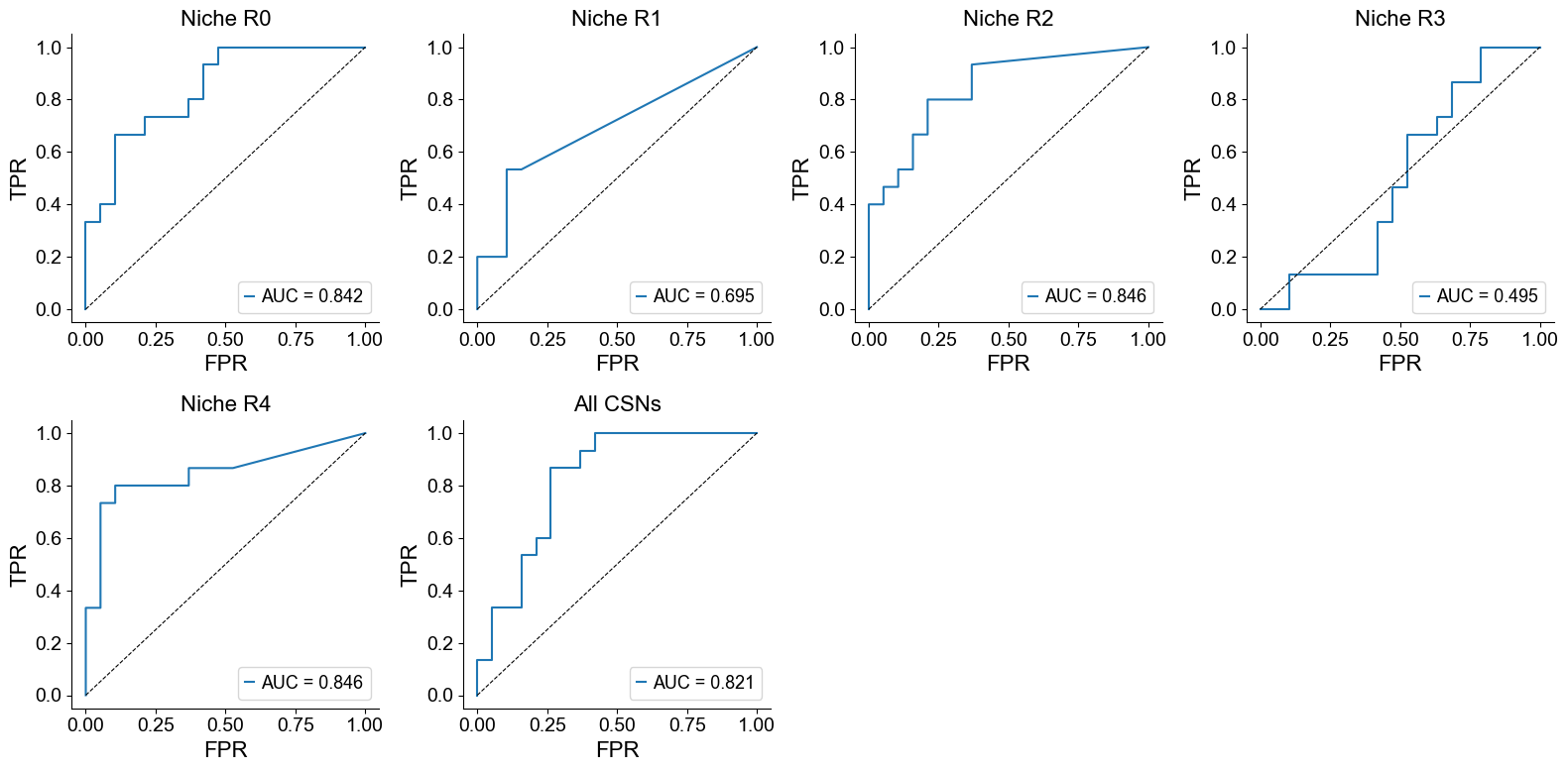
Proportion of a specific CSN across the whole slice
[40]:
ncol = 4
nrow = int(np.ceil((len(csns)+1) / ncol))
fig, axes = plt.subplots(nrow, ncol, figsize=(4*ncol, 4*nrow))
axes = axes.flatten()

for i, roi in enumerate(csns):

    ratios = []
    for cond_name in cond_name_list:
        adata = cond_concat[cond_concat.obs['slice_name'] == cond_name, :].copy()
        roi_ratio = (adata.obs['csn_label'] == roi).mean()
        ratios.append(roi_ratio)

    ratios = np.array(ratios)

    # ROC curve
    fpr, tpr, _ = roc_curve(group_labels, ratios)
    roc_auc = auc(fpr, tpr)

    ax = axes[i]
    ax.plot(fpr, tpr, label=f'AUC = {roc_auc:.3f}')
    ax.plot([0, 1], [0, 1], 'k--', linewidth=0.8)
    ax.set_title(f'Niche {roi}', fontsize=16)
    ax.set_xlabel('FPR', fontsize=16)
    ax.set_ylabel('TPR', fontsize=16)
    ax.grid(False)
    ax.spines['top'].set_visible(False)
    ax.spines['right'].set_visible(False)
    ax.legend(loc='lower right')

    if i == len(csns)-1:
        i += 1
        ratios = []
        for cond_name in cond_name_list:
            adata = cond_concat[cond_concat.obs['slice_name'] == cond_name, :].copy()
            roi_ratio = (adata.obs['csn_label'].isin(csns)).mean()
            ratios.append(roi_ratio)

        ratios = np.array(ratios)

        # ROC curve
        fpr, tpr, _ = roc_curve(group_labels, ratios)
        roc_auc = auc(fpr, tpr)

        ax = axes[i]
        ax.plot(fpr, tpr, label=f'AUC = {roc_auc:.3f}')
        ax.plot([0, 1], [0, 1], 'k--', linewidth=0.8)
        ax.set_title(f'All CSNs', fontsize=16)
        ax.set_xlabel('FPR', fontsize=16)
        ax.set_ylabel('TPR', fontsize=16)
        ax.grid(False)
        ax.spines['top'].set_visible(False)
        ax.spines['right'].set_visible(False)
        ax.legend(loc='lower right')

for j in range(len(csns)+1, nrow*ncol):
    axes[j].axis('off')

plt.tight_layout()
plt.show()
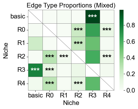
Niche-niche co-localization analysis
Split into two subtypes
[41]:
mixed_slice_name = [f'p{id}' for id in mixed_group]
compart_slice_name = [f'p{id}' for id in compartmentalized_group]
mixed_adata_list = [cond_list[i].copy() for i in range(len(cond_list)) if cond_list[i].obs['slice_name'][0] in mixed_slice_name]
compart_adata_list = [cond_list[i].copy() for i in range(len(cond_list)) if cond_list[i].obs['slice_name'][0] in compart_slice_name]
print('Mixed group adata list length:', len(mixed_adata_list))
print('Compartmentalized group adata list length:', len(compart_adata_list))
Mixed group adata list length: 19
Compartmentalized group adata list length: 15
mixed group
[42]:
csn_labels = ['basic', 'R0', 'R1', 'R2', 'R3', 'R4']
nnc_results_mixed = nnc_enrichment_test(mixed_adata_list,
                                        'csn_label',
                                        niche_summary=csn_labels,
                                        spatial_key='spatial',
                                        cut_percentage=99,
                                        method='fisher',
                                        alpha=0.05,
                                        fdr_method='fdr_by',
                                        log2fc_threshold=1,
                                        prop_threshold=0.01,
                                        verbose=True,
                                        )
nnc_df_mixed, edge_prop_mtx_mixed, n1_count_mixed = nnc_results_mixed

nnc_df_mixed['stars'] = nnc_df_mixed['q-value'].apply(p2stars)

matrix_df = pd.DataFrame(
    data=edge_prop_mtx_mixed,
    index=csn_labels,
    columns=csn_labels,
)

for i in range(matrix_df.shape[0]):
    for j in range(matrix_df.shape[1]):
        if i == j:
            matrix_df.iloc[i, j] = np.nan

stars_df = pd.DataFrame(
    '',
    index=matrix_df.index,
    columns=matrix_df.columns
)

for _, row in nnc_df_mixed[nnc_df_mixed['enrichment']].iterrows():
    n1 = row['niche1']
    n2 = row['niche2']
    if (n1 in stars_df.index) and (n2 in stars_df.columns):
        stars_df.loc[n1, n2] = row['stars']

plt.figure(figsize=(5, 4))

ax  = sns.heatmap(
    matrix_df,
    cmap='Greens',
    # cbar_kws={'label': 'Edge type proportion'},
    linewidths=0.7,
    linecolor='gray',
    # square=True,
)

for i, n1 in enumerate(matrix_df.index):
    for j, n2 in enumerate(matrix_df.columns):
        if i == j:
            ax.plot([i, i+1], [i, i+1], color='gray', linewidth=0.7)
            # ax.plot([i+1, i], [i, i+1], color='gray', linewidth=0.7)
            continue
        star = stars_df.iloc[i, j]
        if star:
            if matrix_df.iloc[i, j] > np.nanmax(matrix_df.values) * 0.7:
                color='white'
            else:
                color='black'
            ax.text(j + 0.5, i + 0.6, star, ha='center', va='center', color=color, fontsize=20, fontweight='bold')

n_rows, n_cols = matrix_df.shape
ax.plot([0, n_cols], [n_rows, n_rows], color='gray', linewidth=0.7, clip_on=False)
ax.plot([n_cols, n_cols], [0, n_rows], color='gray', linewidth=0.7, clip_on=False)

ax.set_xticklabels(ax.get_xticklabels(), rotation=0, ha='center', fontsize=16)
ax.set_yticklabels(ax.get_yticklabels(), rotation=0, ha='right', fontsize=16)
ax.set_ylabel('Niche', fontsize=16)
ax.set_xlabel('Niche', fontsize=16)
ax.set_title('Edge Type Proportions (Mixed)', fontsize=16)
ax.collections[0].colorbar.ax.yaxis.label.set_size(16)
ax.collections[0].colorbar.ax.tick_params(labelsize=16)
ax.grid(False)

plt.tight_layout()
plt.show()
6 niches in total.
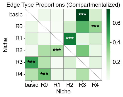
Compartmentalized group
[43]:
csn_labels = ['basic', 'R0', 'R1', 'R2', 'R3', 'R4']
nnc_results_compart = nnc_enrichment_test(compart_adata_list,
                                        'csn_label',
                                        niche_summary=csn_labels,
                                        spatial_key='spatial',
                                        cut_percentage=99,
                                        method='fisher',
                                        alpha=0.05,
                                        fdr_method='fdr_by',
                                        log2fc_threshold=1,
                                        prop_threshold=0.01,
                                        verbose=True,
                                        )
nnc_df_compart, edge_prop_mtx_compart, n1_count_compart = nnc_results_compart

nnc_df_compart['stars'] = nnc_df_compart['q-value'].apply(p2stars)
matrix_df = pd.DataFrame(
    data=edge_prop_mtx_compart,
    index=csn_labels,
    columns=csn_labels,
)

for i in range(matrix_df.shape[0]):
    for j in range(matrix_df.shape[1]):
        if i == j:
            matrix_df.iloc[i, j] = np.nan

stars_df = pd.DataFrame(
    '',
    index=matrix_df.index,
    columns=matrix_df.columns
)

for _, row in nnc_df_compart[nnc_df_compart['enrichment']].iterrows():
    n1 = row['niche1']
    n2 = row['niche2']
    if (n1 in stars_df.index) and (n2 in stars_df.columns):
        stars_df.loc[n1, n2] = row['stars']

plt.figure(figsize=(5, 4))

ax  = sns.heatmap(
    matrix_df,
    cmap='Greens',
    # cbar_kws={'label': 'Edge type proportion'},
    linewidths=0.7,
    linecolor='gray',
    # square=True,
)

for i, n1 in enumerate(matrix_df.index):
    for j, n2 in enumerate(matrix_df.columns):
        if i == j:
            ax.plot([i, i+1], [i, i+1], color='gray', linewidth=0.7)
            # ax.plot([i+1, i], [i, i+1], color='gray', linewidth=0.7)
            continue
        star = stars_df.iloc[i, j]
        if star:
            if matrix_df.iloc[i, j] > np.nanmax(matrix_df.values) * 0.7:
                color='white'
            else:
                color='black'
            ax.text(j + 0.5, i + 0.6, star, ha='center', va='center', color=color, fontsize=20, fontweight='bold')

n_rows, n_cols = matrix_df.shape
ax.plot([0, n_cols], [n_rows, n_rows], color='gray', linewidth=0.7, clip_on=False)
ax.plot([n_cols, n_cols], [0, n_rows], color='gray', linewidth=0.7, clip_on=False)

ax.set_xticklabels(ax.get_xticklabels(), rotation=0, ha='center', fontsize=16)
ax.set_yticklabels(ax.get_yticklabels(), rotation=0, ha='right', fontsize=16)
ax.set_ylabel('Niche', fontsize=16)
ax.set_xlabel('Niche', fontsize=16)
ax.set_title('Edge Type Proportions (Compartmentalized)', fontsize=16)
ax.collections[0].colorbar.ax.yaxis.label.set_size(16)
ax.collections[0].colorbar.ax.tick_params(labelsize=16)
ax.grid(False)

plt.tight_layout()
plt.show()
6 niches in total.
Comparing niche-niche co-localization pattern between mixed group and compartmentalized group
[44]:
edge_prop_mtx_compart_list = []
edge_prop_mtx_mixed_list = []

niche_labels = ['basic', 'R0', 'R1', 'R2', 'R3', 'R4']
n_niches = len(niche_labels)

for i in range(len(compart_adata_list)):
    edge_prop_mtx, _ = cal_nnc_mtx(compart_adata_list[i], 'csn_label', niche_summary=niche_labels, adj_mtx_key='delaunay_adj_mtx')
    edge_prop_mtx_compart_list.append(edge_prop_mtx)

for i in range(len(mixed_adata_list)):
    edge_prop_mtx, _ = cal_nnc_mtx(mixed_adata_list[i], 'csn_label', niche_summary=niche_labels, adj_mtx_key='delaunay_adj_mtx')
    edge_prop_mtx_mixed_list.append(edge_prop_mtx)

nnc_btgroup_df = nnc_between_groups_test(edge_prop_mtx_compart_list,
                                         edge_prop_mtx_mixed_list,
                                         niche_labels,
                                         min_valid=3,
                                         alpha=0.05,
                                         alternative="two-sided",
                                         fdr_method="fdr_bh",
                                         )
nnc_btgroup_df.head()
[44]:
| niche1 | niche2 | mean1 | mean2 | delta_mean | n1_valid | n2_valid | p_value | q_value | rejected | |
|---|---|---|---|---|---|---|---|---|---|---|
| 0 | basic | R0 | 0.050620 | 0.003027 | 0.047593 | 15 | 19 | 0.006082 | 0.021570 | False |
| 1 | basic | R1 | 0.045948 | 0.002907 | 0.043041 | 15 | 19 | 0.105328 | 0.170161 | False |
| 2 | basic | R2 | 0.019912 | 0.000100 | 0.019812 | 15 | 19 | 0.000413 | 0.004131 | False |
| 3 | basic | R3 | 0.764465 | 0.986027 | -0.221562 | 15 | 19 | 0.000078 | 0.001164 | False |
| 4 | basic | R4 | 0.119055 | 0.007939 | 0.111115 | 15 | 19 | 0.002008 | 0.010039 | False |
[45]:
delta_mtx = np.full((n_niches, n_niches), np.nan, dtype=float)
q_mtx = np.full((n_niches, n_niches), np.nan, dtype=float)

for _, r in nnc_btgroup_df.iterrows():
    i = niche_labels.index(r["niche1"])
    j = niche_labels.index(r["niche2"])
    delta_mtx[i, j] = r["delta_mean"]
    q_mtx[i, j] = r["q_value"]

plt.figure(figsize=(5, 4))
ax = sns.heatmap(
    delta_mtx,
    xticklabels=niche_labels,
    yticklabels=niche_labels,
    cmap="coolwarm",
    center=0,
    linewidths=0.5,
    linecolor="white",
    # cbar_kws={"label": r"$\Delta$ edge_prop"}
)
ax.set_title(r"$\Delta$ edge_prop (compartmentalized - mixed)", fontsize=16)
ax.set_xticklabels(ax.get_xticklabels(), rotation=0, ha='center', fontsize=16)
ax.set_yticklabels(ax.get_yticklabels(), rotation=0, ha='right', fontsize=16)
ax.set_ylabel('Niche', fontsize=16)
ax.set_xlabel('Niche', fontsize=16)
ax.collections[0].colorbar.ax.yaxis.label.set_size(16)
ax.collections[0].colorbar.ax.tick_params(labelsize=16)
ax.grid(False)
ax.plot([0, n_niches], [n_niches, n_niches], color='white', linewidth=0.5, clip_on=False)
ax.plot([n_niches, n_niches], [0, n_niches], color='white', linewidth=0.5, clip_on=False)

for i in range(n_niches):
    for j in range(n_niches):
        if i == j: continue
        q = q_mtx[i, j]
        if np.isnan(q): continue
        star = p2stars(q)
        if star != "":
            ax.text(j + 0.5, i + 0.6, star, ha="center", va="center", fontsize=20, color="black", fontweight="bold")

plt.tight_layout()
plt.show()
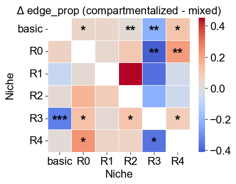
Tumor-immune interaction niche (R3)
Cell-cell interaction analysis for R3
[46]:
cci_results = cci_enrichment_test(cond_list,
                                  'csn_label',
                                  'all_group_name',
                                  niche_summary=['R3'],
                                  spatial_key='spatial',
                                  cut_percentage=99,
                                  method='fisher',
                                  alpha=0.05,
                                  fdr_method='fdr_by',
                                  log2fc_threshold=1,
                                  prop_threshold=0.01,
                                  verbose=True,
                                  )
cci_df, test_norm_list, bg_norm_list, test_edge_count_list, bg_edge_count_list = cci_results
cci_df.head()
1 niches and 16 cell types in total.

Testing niche R3...
Finished!
[46]:
| niche_idx | niche | ct1_idx | ct1 | ct2_idx | ct2 | test_edge_count | bg_edge_count | test_edge_prop | bg_edge_prop | oddsratio | p-value | q-value | log2fc | enrichment | |
|---|---|---|---|---|---|---|---|---|---|---|---|---|---|---|---|
| 0 | 0 | R3 | 0 | B | 0 | B | 345.0 | 14794.0 | 0.002975 | 0.041401 | 0.069090 | 0.000000 | 0.000000 | -3.798676 | False |
| 1 | 0 | R3 | 1 | CD3 T | 0 | B | 254.0 | 771.0 | 0.002190 | 0.002158 | 1.015184 | 0.827408 | 1.000000 | 0.021693 | False |
| 2 | 0 | R3 | 1 | CD3 T | 1 | CD3 T | 275.0 | 782.0 | 0.002371 | 0.002188 | 1.083819 | 0.252054 | 1.000000 | 0.115859 | False |
| 3 | 0 | R3 | 2 | CD4 T | 0 | B | 436.0 | 7673.0 | 0.003760 | 0.021473 | 0.171981 | 0.000000 | 0.000000 | -2.513795 | False |
| 4 | 0 | R3 | 2 | CD4 T | 1 | CD3 T | 515.0 | 1890.0 | 0.004441 | 0.005289 | 0.838931 | 0.000362 | 0.003007 | -0.252146 | False |
[47]:
niche_labels = ['R3']
ct_labels = sorted(adata_concat_new.obs['all_group_name'].unique())

cci_df['stars'] = cci_df['q-value'].apply(p2stars)

figrows = 1
figcols = 1

fig, axes = plt.subplots(figrows, figcols, figsize=(9, 8))

for idx in range(figrows * figcols):

    imgrow = idx // figcols
    imgcol = idx % figcols

    if figcols == 1 and figrows == 1:
        ax = axes
    elif figrows == 1:
        ax = axes[imgcol]
    elif figcols == 1:
        ax = axes[imgrow]
    else:
        ax = axes[imgrow, imgcol]

    if idx >= len(niche_labels):
        ax.axis('off')
        continue

    sub_df = cci_df[cci_df['niche_idx'] == idx]

    matrix_df = pd.DataFrame(
        data=test_norm_list[idx],
        index=ct_labels,
        columns=ct_labels,
    )

    for i in range(matrix_df.shape[0]):
        for j in range(matrix_df.shape[1]):
            if i < j:
                matrix_df.iloc[i, j] = np.nan

    stars_df = pd.DataFrame(
        '',
        index=matrix_df.index,
        columns=matrix_df.columns
    )

    for _, row in sub_df[sub_df['enrichment']].iterrows():
        ct1 = row['ct1']
        ct2 = row['ct2']
        if (ct1 in stars_df.index) and (ct2 in stars_df.columns):
            stars_df.loc[ct1, ct2] = row['stars']

    sns_heatmap = sns.heatmap(
        matrix_df,
        cmap='Oranges',
        mask=matrix_df.isna(),
        # cbar_kws={'label': 'Edge type proportion'},
        # linewidths=0.5,
        # linecolor='gray',
        # square=True,
        ax=ax,
    )

    n_rows, n_cols = matrix_df.shape

    for i, ct1 in enumerate(matrix_df.index):
        ax.plot([0, i+1], [i, i], color='gray', linewidth=0.5, clip_on=False)
        ax.plot([i+1, i+1], [i, n_rows], color='gray', linewidth=0.5, clip_on=False)
        for j, ct2 in enumerate(matrix_df.columns):
            star = stars_df.iloc[i, j]
            if star:
                if matrix_df.iloc[i, j] > np.nanmax(matrix_df.values) * 0.7:
                    color='white'
                else:
                    color='black'
                ax.text(j + 0.5, i + 0.6, star, ha='center', va='center', color=color, fontsize=16, fontweight='bold')

    ax.plot([0, 0], [0, n_rows], color='gray', linewidth=0.5, clip_on=False)
    ax.plot([0, n_cols], [n_rows, n_rows], color='gray', linewidth=0.5, clip_on=False)
    # ax.plot([0, n_cols], [n_rows, n_rows], color='gray', linewidth=0.5, clip_on=False)
    # ax.plot([n_cols, n_cols], [0, n_rows], color='gray', linewidth=0.5, clip_on=False)

    ax.set_xticklabels(ax.get_xticklabels(), rotation=90, ha='center', fontsize=16)
    ax.set_yticklabels(ax.get_yticklabels(), rotation=0, ha='right', fontsize=16)
    ax.set_ylabel('Cell Type', fontsize=16)
    ax.set_xlabel('Cell Type', fontsize=16)
    ax.set_title(f'Niche {niche_labels[idx]}', fontsize=16)
    ax.collections[0].colorbar.ax.yaxis.label.set_size(16)
    ax.collections[0].colorbar.ax.tick_params(labelsize=16)
    ax.grid(False)

plt.tight_layout()
plt.show()
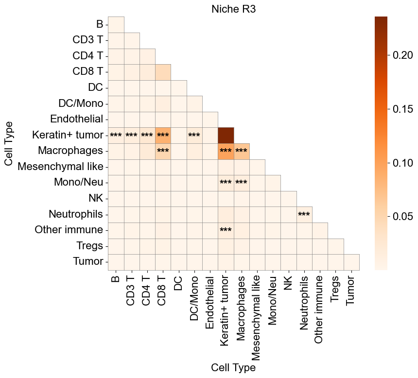
Niche neighborhood classification
[48]:
mix_cell_count = 100
csn_labels = ['basic', 'R0', 'R1', 'R2', 'R3', 'R4']
niche_neigh_rep_dict = {}
for i in range(len(cond_list)):
    adata = cond_list[i].copy()
    if np.sum(adata.obs['csn_label'] == 'R3') < mix_cell_count:
        print(f'Slice {adata.obs["slice_name"][0]} skipped due to low R3 cell count.')
        continue
    edge_prop_mtx, _ = cal_nnc_mtx(adata, 'csn_label', niche_summary=csn_labels, adj_mtx_key='delaunay_adj_mtx')
    rep = np.array(edge_prop_mtx[csn_labels.index('R3'), :], dtype=float)
    niche_neigh_rep_dict[adata.obs['slice_name'][0]] = rep[~np.isnan(rep)]
Slice p18 skipped due to low R3 cell count.
Slice p21 skipped due to low R3 cell count.
Slice p31 skipped due to low R3 cell count.
Slice p33 skipped due to low R3 cell count.
[53]:
from sklearn.metrics.pairwise import cosine_similarity
from scipy.spatial.distance import jensenshannon
from scipy.spatial.distance import squareform
from scipy.cluster.hierarchy import linkage, leaves_list, fcluster
from matplotlib import gridspec
from scipy.cluster.hierarchy import dendrogram

patients = list(niche_neigh_rep_dict.keys())
n_patient = len(patients)
X = np.vstack([niche_neigh_rep_dict[p] for p in patients])  # n_patient x n_feature
edge_prop_df = pd.DataFrame(X, index=patients, columns=csn_labels)

# S = np.zeros((n_patient, n_patient))
# for i in range(n_patient):
#     for j in range(n_patient):
#         S[i, j] = 1 - jensenshannon(X[i], X[j], base=2)

# S = np.corrcoef(X)  # n_patient x n_patient
S = cosine_similarity(X)  # n_patient x n_patient
S_df = pd.DataFrame(S, index=patients, columns=patients)

D = 1.0 - S_df.values
np.fill_diagonal(D, 0.0)
# D = np.sqrt(D)
condensed_D = squareform(D, checks=False)
Z = linkage(condensed_D, method='average', metric='euclidean')

order = leaves_list(Z)
ordered_patients = [patients[i] for i in order]
S_ord = S_df.loc[ordered_patients, ordered_patients]

fig = plt.figure(figsize=(9, 9))
gs = gridspec.GridSpec(2, 2, height_ratios=[1, 6], width_ratios=[18, 1], hspace=0.02, wspace=0.15)

ax_dendro = fig.add_subplot(gs[0, 0])
ax_hm = fig.add_subplot(gs[1, 0])
cax = fig.add_subplot(gs[1, 1])

dendrogram(Z, ax=ax_dendro, color_threshold=0, no_labels=True, link_color_func=lambda k: "black")
ax_dendro.axis("off")

sns.heatmap(
    S_ord,
    xticklabels=ordered_patients,
    yticklabels=ordered_patients,
    cmap="RdBu_r",
    # linewidths=0.5,
    linecolor="white",
    cbar=True,
    ax=ax_hm,
    cbar_ax=cax,
)
ax_dendro.set_title('R3 niche neighborhood similarity heatmap', fontsize=20)
ax_hm.set_xticklabels(ax_hm.get_xticklabels(), rotation=90, ha='center', fontsize=16)
ax_hm.set_yticklabels(ax_hm.get_yticklabels(), rotation=0, ha='right', fontsize=16)
# ax_hm.set_ylabel('Patient', fontsize=16)
# ax_hm.set_xlabel('Patient', fontsize=16)
ax_hm.collections[0].colorbar.ax.yaxis.label.set_size(16)
ax_hm.collections[0].colorbar.ax.tick_params(labelsize=16)
ax_hm.grid(False)

# for label in ax_hm.get_xticklabels():
#     patient_id = label.get_text()
#     if patient_id in slice_color_dict:
#         label.set_color(slice_color_dict[patient_id])
# for label in ax_hm.get_yticklabels():
#     patient_id = label.get_text()
#     if patient_id in slice_color_dict:
#         label.set_color(slice_color_dict[patient_id])

plt.tight_layout()
plt.show()
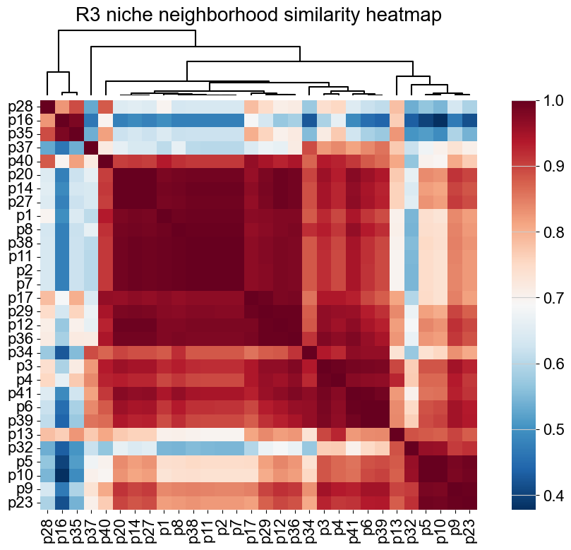
[50]:
labels = fcluster(Z, t=4, criterion="maxclust")
cluster_df = pd.DataFrame({"patient": patients, "cluster": labels})
cluster_counts = cluster_df["cluster"].value_counts()
top2_clusters = cluster_counts.index[:2].tolist()
cluster_top2_df = cluster_df[cluster_df["cluster"].isin(top2_clusters)]

subtype_1_name = cluster_top2_df[cluster_top2_df["cluster"] == top2_clusters[0]]["patient"].tolist()
subtype_2_name = cluster_top2_df[cluster_top2_df["cluster"] == top2_clusters[1]]["patient"].tolist()
print("Subtype 1 patients (n={}):".format(len(subtype_1_name)), subtype_1_name)
print("Subtype 2 patients (n={}):".format(len(subtype_2_name)), subtype_2_name)

df1 = edge_prop_df.loc[subtype_1_name].copy()
df2 = edge_prop_df.loc[subtype_2_name].copy()
df1["Subtype"] = "Subtype 1"
df2["Subtype"] = "Subtype 2"
df_long = pd.concat([df1, df2], axis=0)
df_long = df_long.reset_index().rename(columns={"index": "patient"})
df_long = df_long.melt(id_vars=["patient", "Subtype"], value_vars=csn_labels, var_name="Neighbor_niche", value_name="Edge_prop")
Subtype 1 patients (n=20): ['p1', 'p2', 'p3', 'p4', 'p6', 'p7', 'p8', 'p11', 'p12', 'p14', 'p17', 'p20', 'p27', 'p29', 'p34', 'p36', 'p38', 'p39', 'p40', 'p41']
Subtype 2 patients (n=6): ['p5', 'p9', 'p10', 'p13', 'p23', 'p32']
[51]:
from scipy.stats import mannwhitneyu
from matplotlib.patches import Patch

subtype_color_dict = {"Subtype 1": "#D8B365", "Subtype 2": "#A6CEE3",  }

plt.figure(figsize=(1.7 * len(csn_labels), 4))
ax = plt.gca()

x_pos = np.arange(len(csn_labels))
offset = 0.22

# boxplot: Subtype 1
sns.boxplot(data=df_long[df_long["Subtype"] == "Subtype 1"], x="Neighbor_niche", y="Edge_prop",
            order=csn_labels, color=subtype_color_dict["Subtype 1"], width=0.35, ax=ax, positions=x_pos - offset, showfliers=False)

# boxplot: Subtype 2
sns.boxplot(data=df_long[df_long["Subtype"] == "Subtype 2"], x="Neighbor_niche", y="Edge_prop",
            order=csn_labels, color=subtype_color_dict["Subtype 2"], width=0.35, ax=ax, positions=x_pos + offset, showfliers=False)
# scatter
sns.stripplot(data=df_long, x="Neighbor_niche", y="Edge_prop", hue="Subtype", dodge=True, jitter=True, size=7, alpha=0.7,
              edgecolor="black", linewidth=1, palette={"Subtype 1": "white", "Subtype 2": "white"}, ax=ax)

stats_res = []
for i, niche in enumerate(csn_labels):
    x1 = df_long[(df_long["Neighbor_niche"] == niche) & (df_long["Subtype"] == "Subtype 1")]["Edge_prop"]
    x2 = df_long[(df_long["Neighbor_niche"] == niche) & (df_long["Subtype"] == "Subtype 2")]["Edge_prop"]

    y_max = max(x1.max(), x2.max())

    _, p = mannwhitneyu(x1, x2, alternative="two-sided")
    stats_res.append({"Neighbor_niche": niche, "pvalue": p})
    ax.text(i, y_max + 0.05, f"p = {p:.2e}" if p == p else "n.a.", ha="center", va="bottom", fontsize=16)

legend_elements = [
    Patch(facecolor=subtype_color_dict["Subtype 1"], edgecolor="black", label="Subtype 1"),
    Patch(facecolor=subtype_color_dict["Subtype 2"], edgecolor="black", label="Subtype 2")
]
ax.legend(handles=legend_elements, frameon=False, fontsize=16, loc="upper right")

ax.set_ylabel("Edge proportion", fontsize=16)
ax.set_xlabel("")
ax.set_xticklabels(csn_labels, rotation=0, ha="center", fontsize=16)
ax.tick_params(axis="y", labelsize=16)
ax.spines["top"].set_visible(False)
ax.spines["right"].set_visible(False)
ax.grid(False)

plt.tight_layout()
plt.show()
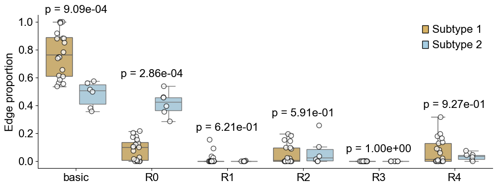
Differential expression analysis
Keratin+ tumor
[56]:
from scipy.stats import wilcoxon, mannwhitneyu
from statannotations.Annotator import Annotator
np.random.seed(1234)

noi = 'R3'
ctoi = ['Keratin+ tumor']
markers = cond_concat_new.var_names.tolist()
markers = ['Ki67', 'phospho-S6']
n_markers = len(markers)

avg_expr_noi_subtype_1 = [[] for _ in range(n_markers)]
avg_expr_noi_subtype_2 = [[] for _ in range(n_markers)]
# avg_expr_other_subtype_1 = [[] for _ in range(n_markers)]
# avg_expr_other_subtype_2 = [[] for _ in range(n_markers)]
# avg_expr_whole_subtype_1 = [[] for _ in range(n_markers)]
# avg_expr_whole_subtype_2 = [[] for _ in range(n_markers)]
# new_marker_list = []

for i, slice_name in enumerate(subtype_1_name):
    adata = cond_concat_new[cond_concat_new.obs['slice_name'] == slice_name, :].copy()
    adata_noi = adata[(adata.obs['all_group_name'].isin(ctoi)) & (adata.obs['csn_label'] == noi), :].copy()
    # adata_other = adata[(adata.obs['all_group_name'].isin(ctoi)) & (adata.obs['csn_label'] != noi), :].copy()
    # adata_whole = adata[adata.obs['all_group_name'].isin(ctoi), :].copy()
    for j, marker in enumerate(markers):
        avg_expr_noi_subtype_1[j].append(np.mean(adata_noi[:, marker].X > 0.5))
        # avg_expr_other_subtype_1[j].append(np.mean(adata_other[:, marker].X > 0.5))
        # avg_expr_whole_subtype_1[j].append(np.mean(adata_whole[:, marker].X > 0.5))

for i, slice_name in enumerate(subtype_2_name):
    adata = cond_concat_new[cond_concat_new.obs['slice_name'] == slice_name, :].copy()
    adata_noi = adata[(adata.obs['all_group_name'].isin(ctoi)) & (adata.obs['csn_label'] == noi), :].copy()
    # adata_other = adata[(adata.obs['all_group_name'].isin(ctoi)) & (adata.obs['csn_label'] != noi), :].copy()
    # adata_whole = adata[adata.obs['all_group_name'].isin(ctoi), :].copy()
    for j, marker in enumerate(markers):
        avg_expr_noi_subtype_2[j].append(np.mean(adata_noi[:, marker].X > 0.5))
        # avg_expr_other_subtype_2[j].append(np.mean(adata_other[:, marker].X > 0.5))
        # avg_expr_whole_subtype_2[j].append(np.mean(adata_whole[:, marker].X > 0.5))

### noi
res = []
for j, marker in enumerate(markers):
    x1 = np.array(avg_expr_noi_subtype_1[j], dtype=float)
    x2 = np.array(avg_expr_noi_subtype_2[j], dtype=float)
    u, p = mannwhitneyu(x1, x2, alternative="two-sided")
    res.append({"marker": marker, "pvalue": p, "U": u, "n1": len(x1), "n2": len(x2)})
res_df_noi = pd.DataFrame(res)
alpha = 0.05
sig_df_noi = res_df_noi[res_df_noi["pvalue"] < alpha]#.sort_values("pvalue")
print(f"Significant markers ({noi}): {sig_df_noi.shape[0]} / {len(markers)}")
sig_markers = sig_df_noi["marker"].tolist()

# ### other
# res = []
# for j, marker in enumerate(markers):
#     x1 = np.array(avg_expr_other_subtype_1[j], dtype=float)
#     x2 = np.array(avg_expr_other_subtype_2[j], dtype=float)
#     u, p = mannwhitneyu(x1, x2, alternative="two-sided")
#     res.append({"marker": marker, "pvalue": p, "U": u, "n1": len(x1), "n2": len(x2)})
# res_df_other = pd.DataFrame(res)
# alpha = 0.05
# print(f"Significant markers (Other): {res_df_other[res_df_other['pvalue'] < alpha].shape[0]} / {len(markers)}")

# ### whole
# res = []
# for j, marker in enumerate(markers):
#     x1 = np.array(avg_expr_whole_subtype_1[j], dtype=float)
#     x2 = np.array(avg_expr_whole_subtype_2[j], dtype=float)
#     u, p = mannwhitneyu(x1, x2, alternative="two-sided")
#     res.append({"marker": marker, "pvalue": p, "U": u, "n1": len(x1), "n2": len(x2)})
# res_df_whole = pd.DataFrame(res)
# alpha = 0.05
# print(f"Significant markers (Whole): {res_df_whole[res_df_whole['pvalue'] < alpha].shape[0]} / {len(markers)}")

if len(sig_markers) == 0:
    print("No significant markers under the chosen threshold.")
else:
    n_plot = len(sig_markers)
    if n_plot > 5:
        ncol = 5
    else:
        ncol = n_plot
    nrow = int(np.ceil(n_plot / ncol))

    ### noi
    fig, axes = plt.subplots(nrow, ncol, figsize=(3*ncol, 3.5*nrow))
    axes = np.array(axes).flatten()

    for k, marker in enumerate(sig_markers):
        j = markers.index(marker)
        vals_subtype_1 = avg_expr_noi_subtype_1[j]
        vals_subtype_2 = avg_expr_noi_subtype_2[j]
        ax = axes[k]

        df_plot = pd.DataFrame({
            "expr": np.concatenate([vals_subtype_1, vals_subtype_2]),
            "group": ["Subtype 1"]*len(vals_subtype_1) + ["Subtype 2"]*len(vals_subtype_2),
            # "patient": subtype_1_name + subtype_2_name
        })
        # print(df_plot.sort_values("expr", ascending=False).head(5))

        colors = [subtype_color_dict["Subtype 1"], subtype_color_dict["Subtype 2"]]
        sns.boxplot(data=df_plot, x="group", y="expr", ax=ax, palette=subtype_color_dict, width=0.5, showfliers=False)
        # sns.violinplot(data=df_plot, x="group", y="expr", ax=ax, palette=subtype_color_dict, inner='box', cut=1)
        sns.stripplot(data=df_plot, x="group", y="expr", ax=ax, jitter=True, size=7, alpha=0.7, color="white", edgecolor="black", linewidth=1)

        pv = sig_df_noi.set_index("marker").loc[marker, "pvalue"]

        ax.set_xticklabels(["Subtype 1", "Subtype 2"], fontsize=14)
        ax.tick_params(axis="y", labelsize=14)
        ax.set_title(f"{marker}\np = {pv:.3e}", fontsize=14)
        ax.set_ylabel("Mean Scaled Expression", fontsize=14)
        ax.set_xlabel("")
        ax.spines["right"].set_visible(False)
        ax.spines["top"].set_visible(False)
        ax.grid(False)

    for ax in axes[n_plot:]:
        ax.axis("off")

    plt.suptitle(f"{ctoi[0]} (R3)", fontsize=16)
    plt.tight_layout()
    plt.show()
Significant markers (R3): 2 / 2
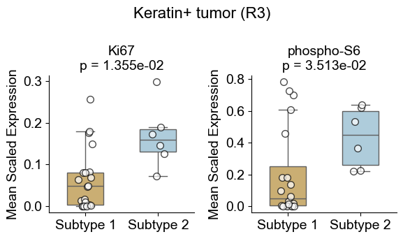
CD8 T cell
[57]:
from scipy.stats import wilcoxon, mannwhitneyu
from statannotations.Annotator import Annotator
np.random.seed(1234)

noi = 'R3'
ctoi = ['CD8 T']
markers = cond_concat_new.var_names.tolist()
markers = ['HLA-DR']
n_markers = len(markers)

avg_expr_noi_subtype_1 = [[] for _ in range(n_markers)]
avg_expr_noi_subtype_2 = [[] for _ in range(n_markers)]
# avg_expr_other_subtype_1 = [[] for _ in range(n_markers)]
# avg_expr_other_subtype_2 = [[] for _ in range(n_markers)]
# avg_expr_whole_subtype_1 = [[] for _ in range(n_markers)]
# avg_expr_whole_subtype_2 = [[] for _ in range(n_markers)]
# new_marker_list = []

for i, slice_name in enumerate(subtype_1_name):
    adata = cond_concat_new[cond_concat_new.obs['slice_name'] == slice_name, :].copy()
    adata_noi = adata[(adata.obs['all_group_name'].isin(ctoi)) & (adata.obs['csn_label'] == noi), :].copy()
    # adata_other = adata[(adata.obs['all_group_name'].isin(ctoi)) & (adata.obs['csn_label'] != noi), :].copy()
    # adata_whole = adata[adata.obs['all_group_name'].isin(ctoi), :].copy()
    for j, marker in enumerate(markers):
        avg_expr_noi_subtype_1[j].append(np.mean(adata_noi[:, marker].X))
        # avg_expr_other_subtype_1[j].append(np.mean(adata_other[:, marker].X))
        # avg_expr_whole_subtype_1[j].append(np.mean(adata_whole[:, marker].X))

for i, slice_name in enumerate(subtype_2_name):
    adata = cond_concat_new[cond_concat_new.obs['slice_name'] == slice_name, :].copy()
    adata_noi = adata[(adata.obs['all_group_name'].isin(ctoi)) & (adata.obs['csn_label'] == noi), :].copy()
    # adata_other = adata[(adata.obs['all_group_name'].isin(ctoi)) & (adata.obs['csn_label'] != noi), :].copy()
    # adata_whole = adata[adata.obs['all_group_name'].isin(ctoi), :].copy()
    for j, marker in enumerate(markers):
        avg_expr_noi_subtype_2[j].append(np.mean(adata_noi[:, marker].X))
        # avg_expr_other_subtype_2[j].append(np.mean(adata_other[:, marker].X))
        # avg_expr_whole_subtype_2[j].append(np.mean(adata_whole[:, marker].X))

### noi
res = []
for j, marker in enumerate(markers):
    x1 = np.array(avg_expr_noi_subtype_1[j], dtype=float)
    x2 = np.array(avg_expr_noi_subtype_2[j], dtype=float)
    u, p = mannwhitneyu(x1, x2, alternative="two-sided")
    res.append({"marker": marker, "pvalue": p, "U": u, "n1": len(x1), "n2": len(x2)})
res_df_noi = pd.DataFrame(res)
alpha = 0.05
sig_df_noi = res_df_noi[res_df_noi["pvalue"] < alpha]#.sort_values("pvalue")
print(f"Significant markers ({noi}): {sig_df_noi.shape[0]} / {len(markers)}")
sig_markers = sig_df_noi["marker"].tolist()

if len(sig_markers) == 0:
    print("No significant markers under the chosen threshold.")
else:
    n_plot = len(sig_markers)
    if n_plot > 5:
        ncol = 5
    else:
        ncol = n_plot
    nrow = int(np.ceil(n_plot / ncol))

    ### noi
    fig, axes = plt.subplots(nrow, ncol, figsize=(3*ncol, 3.5*nrow))
    axes = np.array(axes).flatten()

    for k, marker in enumerate(sig_markers):
        j = markers.index(marker)
        vals_subtype_1 = avg_expr_noi_subtype_1[j]
        vals_subtype_2 = avg_expr_noi_subtype_2[j]
        ax = axes[k]

        df_plot = pd.DataFrame({
            "expr": np.concatenate([vals_subtype_1, vals_subtype_2]),
            "group": ["Subtype 1"]*len(vals_subtype_1) + ["Subtype 2"]*len(vals_subtype_2),
            # "patient": subtype_1_name + subtype_2_name
        })
        # print(df_plot.sort_values("expr", ascending=False).head(5))

        colors = [subtype_color_dict["Subtype 1"], subtype_color_dict["Subtype 2"]]
        sns.boxplot(data=df_plot, x="group", y="expr", ax=ax, palette=subtype_color_dict, width=0.5, showfliers=False)
        # sns.violinplot(data=df_plot, x="group", y="expr", ax=ax, palette=subtype_color_dict, inner='box', cut=1)
        sns.stripplot(data=df_plot, x="group", y="expr", ax=ax, jitter=True, size=7, alpha=0.7, color="white", edgecolor="black", linewidth=1)

        pv = sig_df_noi.set_index("marker").loc[marker, "pvalue"]

        ax.set_xticklabels(["Subtype 1", "Subtype 2"], fontsize=14)
        ax.tick_params(axis="y", labelsize=14)
        ax.set_title(f"{marker}\np = {pv:.3e}", fontsize=14)
        ax.set_ylabel("Mean Scaled Expression", fontsize=14)
        ax.set_xlabel("")
        ax.spines["right"].set_visible(False)
        ax.spines["top"].set_visible(False)
        ax.grid(False)

    for ax in axes[n_plot:]:
        ax.axis("off")

    plt.suptitle(f"{ctoi[0]} (R3)", fontsize=16)
    plt.tight_layout()
    plt.show()
Significant markers (R3): 1 / 1
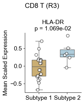
Survival analysis
[58]:
meta = pd.read_csv(data_dir + 'survival_data.csv', header=0, index_col=None)
meta.head()
[58]:
| InternalId | Survival_days | Censored | Event | DONOR_NO | |
|---|---|---|---|---|---|
| 0 | 1 | 2612 | 0 | 1 | 30824 |
| 1 | 2 | 745 | 0 | 1 | 30805 |
| 2 | 3 | 3130 | 1 | 0 | 30812 |
| 3 | 4 | 2523 | 1 | 0 | 30838 |
| 4 | 5 | 1683 | 1 | 0 | 30865 |
Using the proportion of niche R0 as an indicator to classify slices into two subgroups
[60]:
from lifelines import CoxPHFitter
from lifelines import KaplanMeierFitter
from lifelines.statistics import logrank_test

cold_group = [15, 19, 22, 24, 25, 26]  # 6
mixed_group = [1, 2, 7, 8, 11, 12, 13, 14, 17, 18, 20, 21, 23, 27, 29, 31, 33, 38, 39]  # 19
compartmentalized_group = [3, 4, 5, 6, 9, 10, 16, 28, 32, 34, 35, 36, 37, 40, 41]  #15

roi = 'R0'
thres_list = [0, 0.001, 0.003, 0.005, 0.01, 0.03,]
# thres = 0.03

fig, axes = plt.subplots(2, 3, figsize=(20, 10))
axes = axes.flatten()

for idx, thres in enumerate(thres_list):
    rows = []
    for i in range(1, 42):
        if i == 30: continue
        row = meta[meta['InternalId'] == i]
        if row.empty: continue
        survival = row['Survival_days'].iloc[0]
        event = row['Event'].iloc[0]

        if i in cold_group:
            continue
            # adata = adata_concat_new[adata_concat_new.obs['slice_name'] == f'p{i}', :].copy()
        else:
            adata = cond_concat_new[cond_concat_new.obs['slice_name'] == f'p{i}', :].copy()
        roi_ratio = (adata.obs['csn_label'] == roi).mean()

        rows.append({
            'id': i,
            'duration': survival/365,
            'event': event,
            'prop': roi_ratio
        })
        # print(survival, roi_ratio)

    df = pd.DataFrame(rows)
    df['group'] = (df['prop'] > thres)

    cph = CoxPHFitter()
    cph.fit(df, duration_col='duration', event_col='event', formula='group')
    hr = cph.hazard_ratios_['group']
    cox_pval = cph.summary.loc['group', 'p']

    group_high = df[df['group'] == 1]
    group_low = df[df['group'] == 0]

    # print(f"Threshold: {thres}")
    # print("High group IDs:", df[df['group'] == 1]['id'].tolist())
    # print("Low group IDs:", df[df['group'] == 0]['id'].tolist())

    kmf = KaplanMeierFitter()
    results = logrank_test(group_high['duration'], group_low['duration'],
                        event_observed_A=group_high['event'],
                        event_observed_B=group_low['event'])
    logrank_pval = results.p_value

    ax = axes[idx]
    kmf.fit(group_high['duration'], group_high['event'], label=f"high proportion n={df['group'].sum()}")
    kmf.plot_survival_function(ax=ax, linewidth=2.5, ci_show=False, show_censors=True,
                               censor_styles={'marker': '+', 'ms': 12, 'mew': 2,})

    kmf.fit(group_low['duration'], group_low['event'], label=f"low proportion n={df.shape[0] - df['group'].sum()}")
    kmf.plot_survival_function(ax=ax, linewidth=2.5, ci_show=False, show_censors=True,
                               censor_styles={'marker': '+', 'ms': 12, 'mew': 2,})

    ax.text(x=0.7, y=0.30, s=f'HR={hr:.2f}', fontsize=14, transform=ax.transAxes)
    ax.text(x=0.7, y=0.25, s=f'Cox p={cox_pval:.3f}', fontsize=14, transform=ax.transAxes)
    ax.text(x=0.7, y=0.20, s=f'Log-rank p={logrank_pval:.3f}', fontsize=14, transform=ax.transAxes)
    ax.set_title(f'Kaplan-Meier Curve (threshold={thres})', fontsize=18)
    ax.set_xlabel('Years', fontsize=18)
    ax.set_ylabel('Survival', fontsize=18)
    ax.legend(loc='lower left', fontsize=16)

    ax.grid(False)
    ax.spines['right'].set_visible(False)
    ax.spines['top'].set_visible(False)

plt.tight_layout()
plt.show()
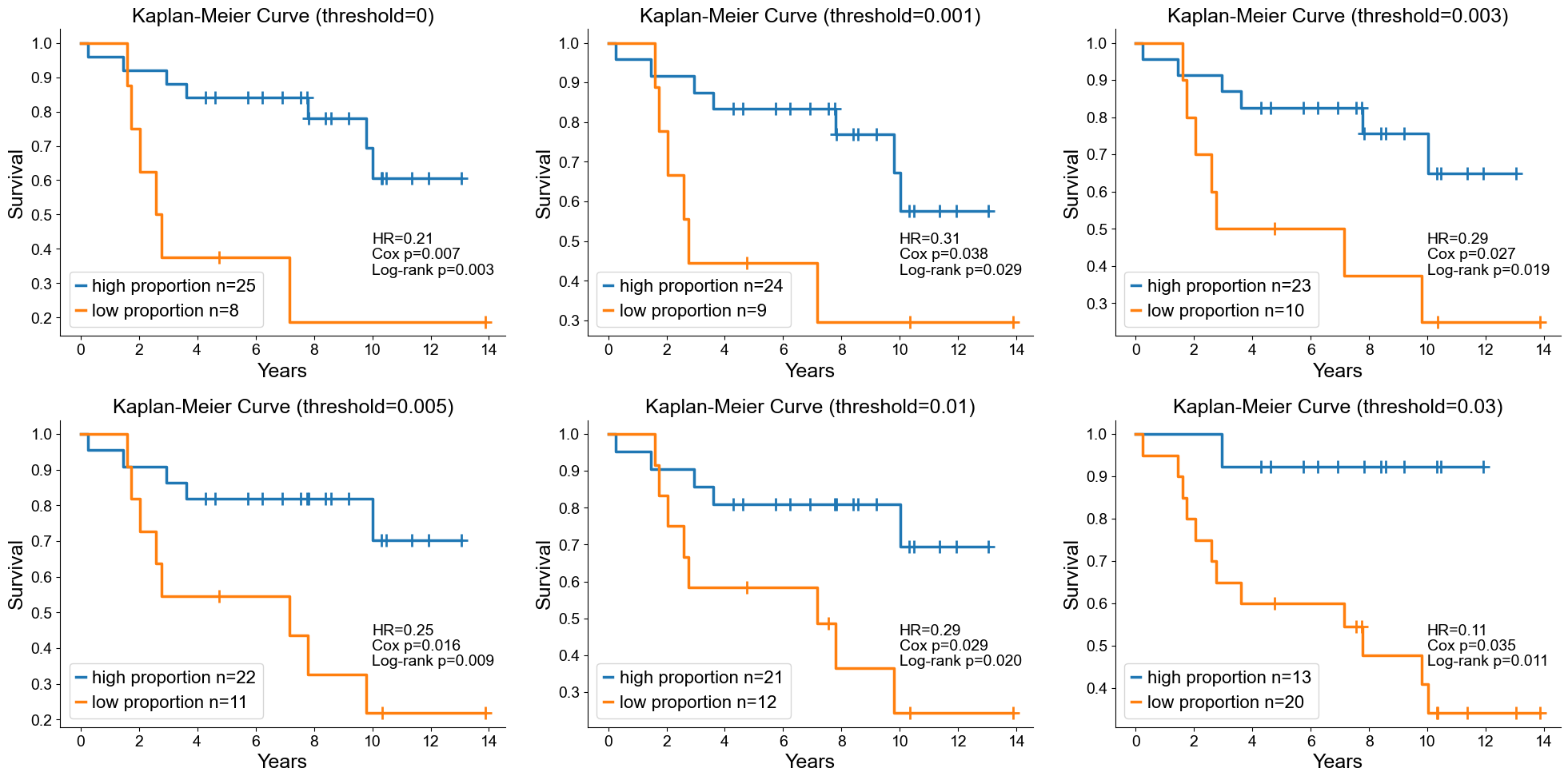
Using the proportion of macrophage as an indicator to classify slices into two subgroups
[61]:
ctoi = 'Macrophages'
thres_list = [0.06, 0.07, 0.075, 0.078, 0.08, 0.117]

fig, axes = plt.subplots(2, 3, figsize=(20, 10))
axes = axes.flatten()

for idx, thres in enumerate(thres_list):
    rows = []
    for i in range(1, 42):
        if i == 30: continue
        row = meta[meta['InternalId'] == i]
        if row.empty: continue
        survival = row['Survival_days'].iloc[0]
        event = row['Event'].iloc[0]

        if i in cold_group:
            continue
            # adata = adata_concat_new[adata_concat_new.obs['slice_name'] == f'p{i}', :].copy()
        else:
            adata = cond_concat_new[cond_concat_new.obs['slice_name'] == f'p{i}', :].copy()
        ctoi_ratio = (adata.obs['all_group_name'] == ctoi).mean()

        rows.append({
            'id': i,
            'duration': survival/365,
            'event': event,
            'prop': ctoi_ratio
        })
        # print(survival, ctoi_ratio)

    df = pd.DataFrame(rows)
    df['group'] = (df['prop'] > thres)

    cph = CoxPHFitter()
    cph.fit(df, duration_col='duration', event_col='event', formula='group')
    hr = cph.hazard_ratios_['group']
    cox_pval = cph.summary.loc['group', 'p']

    group_high = df[df['group'] == 1]
    group_low = df[df['group'] == 0]

    kmf = KaplanMeierFitter()
    results = logrank_test(group_high['duration'], group_low['duration'],
                        event_observed_A=group_high['event'],
                        event_observed_B=group_low['event'])
    logrank_pval = results.p_value

    ax = axes[idx]
    kmf.fit(group_high['duration'], group_high['event'], label=f"high proportion n={df['group'].sum()}")
    kmf.plot_survival_function(ax=ax, linewidth=2.5, ci_show=False, show_censors=True,
                               censor_styles={'marker': '+', 'ms': 12, 'mew': 2,})

    kmf.fit(group_low['duration'], group_low['event'], label=f"low proportion n={df.shape[0] - df['group'].sum()}")
    kmf.plot_survival_function(ax=ax, linewidth=2.5, ci_show=False, show_censors=True,
                               censor_styles={'marker': '+', 'ms': 12, 'mew': 2,})

    ax.text(x=0.70, y=0.40, s=f'HR={hr:.2f}', fontsize=14, transform=ax.transAxes)
    ax.text(x=0.70, y=0.35, s=f'Cox p={cox_pval:.3f}', fontsize=14, transform=ax.transAxes)
    ax.text(x=0.70, y=0.30, s=f'Log-rank p={logrank_pval:.3f}', fontsize=14, transform=ax.transAxes)
    ax.set_title(f'Kaplan-Meier Curve', fontsize=18)
    ax.set_xlabel('Years', fontsize=18)
    ax.set_ylabel('Survival', fontsize=18)
    ax.legend(loc='lower left', fontsize=16)

    ax.grid(False)
    ax.spines['right'].set_visible(False)
    ax.spines['top'].set_visible(False)

plt.tight_layout()
plt.show()