Tutorial for Xenium PF dataset
Need additional packages: scanpy seaborn gseapy statannotations pyslingshot
[1]:
%reload_ext autoreload
%autoreload 2

import os
import time
import gseapy as gp
import scanpy as sc
import pandas as pd
import numpy as np
import anndata as ad
import seaborn as sns
import matplotlib.pyplot as plt
import matplotlib.patches as mpatches
from matplotlib.lines import Line2D
import matplotlib.lines as mlines

from Harmonics import *

import warnings
warnings.filterwarnings("ignore")

sc.settings.verbosity = 0
sc.settings.set_figure_params(dpi=30, dpi_save=500)

from matplotlib import rcParams
rcParams["figure.dpi"] = 30
rcParams["savefig.dpi"] = 500
rcParams['pdf.fonttype'] = 42
rcParams['svg.fonttype'] = 'none'
rcParams['ps.fonttype'] = 42
rcParams['font.family'] = 'Arial'
rcParams['savefig.transparent'] = True
[ ]:
data_dir = '../../../Data/Spatial/Transcriptomics/Xenium_PF_Vannan2025/processed/'
save_dir = '../../results/Xenium_PF_Vannan2025/Harmonics/'
# result_dir = '../../results/Xenium_PF_Vannan2025/fig/'
if not os.path.exists(save_dir):
    os.makedirs(save_dir)
# if not os.path.exists(result_dir):
#     os.makedirs(result_dir)
Define the function to change p values to corresponding star representation, used to show the results of additional tests implemented in Harmonics
[3]:
def p2stars(p):
    if p < 0.001:
        return '***'
    elif p < 0.01:
        return '**'
    elif p < 0.05:
        return '*'
    else:
        return ''
Load dataset
One sample with pathology percentage labeled as 20% is not included since it is even greater than some disease samples
[6]:
ctr_name_list = ['THD0008', 'THD0011', 'VUHD038', 'VUHD049', 'VUHD069', 'VUHD090', 'VUHD095', 'VUHD113', 'VUHD116A', 'VUHD116B',]
cond_name_list = ['TILD028LA', 'TILD049MA', 'TILD080LA', 'TILD111LA', 'TILD113LA', 'TILD117LA', 'TILD117MA1', 'TILD117MA2',
                  'TILD130LA', 'TILD167LA', 'TILD175MA', 'TILD299MA', 'TILD315MA', 'VUILD102LA', 'VUILD102MA', 'VUILD104MA1',
                  'VUILD104MA2', 'VUILD105MA1', 'VUILD105MA2', 'VUILD106MA', 'VUILD107MA', 'VUILD110LA', 'VUILD115MA', 'VUILD141MA',
                  'VUILD142MA', 'VUILD48LA1', 'VUILD48LA2', 'VUILD49LA', 'VUILD58MA', 'VUILD78LA', 'VUILD78MA', 'VUILD91LA',
                  'VUILD91MA', 'VUILD96LA', 'VUILD96MA']
confused_samples = ['THD0011', 'VUHD038', 'VUHD090']  # healthy sample with non-zero pathology percentage
less_affe_list = ['TILD028LA', 'TILD080LA', 'TILD111LA', 'TILD113LA', 'TILD117LA', 'TILD130LA', 'TILD167LA', 'VUILD102LA', 'VUILD110LA',
                  'VUILD48LA1', 'VUILD48LA2', 'VUILD49LA', 'VUILD78LA', 'VUILD91LA', 'VUILD96LA']
more_affe_list = ['TILD049MA', 'TILD117MA1', 'TILD117MA2', 'TILD175MA', 'TILD299MA', 'TILD315MA', 'VUILD102MA', 'VUILD104MA1', 'VUILD104MA2',
                  'VUILD105MA1', 'VUILD105MA2', 'VUILD106MA', 'VUILD107MA', 'VUILD115MA', 'VUILD141MA', 'VUILD142MA', 'VUILD58MA', 'VUILD78MA',
                  'VUILD91MA', 'VUILD96MA']

ctr_list = []
cond_list = []
for slice_name in ctr_name_list:
    if slice_name == 'THD0011':  # this sample is not included since its pathology percentage is 20%, even greater than some disease samples
        continue
    adata = ad.read_h5ad(data_dir + slice_name + '.h5ad')
    ctr_list.append(adata)
ctr_name_list.remove('THD0011')
for slice_name in cond_name_list:
    adata = ad.read_h5ad(data_dir + slice_name + '.h5ad')
    cond_list.append(adata)
Run model
Instantiate Harmonics
[5]:
model = Harmonics_Model(ctr_list,
                        ctr_name_list,
                        cond_list=cond_list,
                        cond_name_list=cond_name_list,
                        concat_label='slice_name',  # default
                        proportion_label=None,  # default
                        seed=1234,  # default
                        parallel=True,  # default
                        verbose=True,  # default
                        )
Control set comprises 9 slices, 199773 cells/spots in total.
Condition set comprises 35 slices, 1405182 cells/spots in total.
Preprocess the data (Generating the connection graph and calculating neighborhood cell type destribution for cells). n_step is set to 2 since we expect to discover highly non-convex structures
[6]:
model.preprocess(ct_key='final_CT',
                 spatial_key='spatial',  # default
                 method='joint',  # default
                 n_step=2,  # set to 2 since we expect to discover highly non-convex structures
                 n_neighbors=20,  # default
                 cut_percentage=99,  # default
                 )
Generating Delaunay neighbor graph...
0%| | 0/44 [00:00<?, ?it/s]100%|██████████| 44/44 [00:31<00:00, 1.40it/s]
All done!

Performing graph completion...
100%|██████████| 44/44 [04:10<00:00, 5.70s/it]
All done!

The cell types of interest are:
AT1
AT2
Activated Fibrotic FBs
Adventitial FBs
Alveolar FBs
Alveolar Macrophages
Arteriole
B cells
Basal
Basophils
CD4+ T-cells
CD8+ T-cells
Capillary
Goblet
Inflammatory FBs
Interstitial Macrophages
KRT5-/KRT17+
Langerhans cells
Lymphatic
Macrophages - IFN-activated
Mast
Mesothelial
Migratory DCs
Monocytes/MDMs
Multiciliated
Myofibroblasts
NK/NKT
Neutrophils
PNEC
Plasma
Proliferating AT2
Proliferating Airway
Proliferating B cells
Proliferating FBs
Proliferating Myeloid
Proliferating NK/NKT
Proliferating T-cells
RASC
SMCs/Pericytes
SPP1+ Macrophages
Secretory
Subpleural FBs
Transitional AT2
Tregs
Venous
cDCs
pDCs

Generating one-hot matrix...
100%|██████████| 44/44 [00:01<00:00, 23.39it/s]
All done!

Dataset comprises 47 cell types.

Calculating cell type distribution for microenvironments...
Microenvironments comprise 21.23 cells/spots on average.
Minimum: 20, Maximum: 66
Perform overclustered initialization on the cell type distributions of cell neighborhoods for the control group. Resulting in Qmax niches. The distributions of niches are also computed.
[7]:
model.initialize_clusters(dim_reduction=True,  # default
                          explained_var=None,  # default
                          n_components=None,  # default
                          n_components_max=100,  # default
                          standardize=True,  # default
                          method='kmeans',  # default
                          Qmax=20,  # default
                          )
Performing dimension reduction...
Returning 47 principal components.

Initializing niches...
20 initial niches defined.
Perform hierarchical distribution matching for the control group to reduce the niche number to no less than Qmin. This step results in niche assignment under a sequence of different niche numbers (usually from Qmax to Qmin).
[ ]:
model.hier_dist_match(assign_metric='jsd',  # default
                      weighted_merge=True,  # default
                      max_iters=100,  # default
                      tol=1e-4,  # default
                      test_kmeans=False,  # default
                      Qmin=2,  # default
                      )
Starting from 20 cell niches...

Assigning cells to cell niche...
Current state: [0, 1, 2, 3, 4, 5, 6, 7, 8, 9, 10, 11, 12, 13, 14, 15, 16, 17, 18, 19]
100%|██████████| 100/100 [00:35<00:00, 2.84it/s]
Unconverged at iteration 100!
20 cell niches left.
Merging cell niche 18 and cell niche 14...
Done!

Assigning cells to cell niche...
Current state: [0, 1, 2, 3, 4, 5, 6, 7, 8, 9, 10, 11, 12, 13, 15, 16, 17, 18, 19]
100%|██████████| 100/100 [00:32<00:00, 3.09it/s]
Unconverged at iteration 100!
19 cell niches left.
Merging cell niche 2 and cell niche 18...
Done!

Assigning cells to cell niche...
Current state: [0, 1, 2, 3, 4, 5, 6, 7, 8, 9, 10, 11, 12, 13, 15, 16, 17, 19]
100%|██████████| 100/100 [00:31<00:00, 3.21it/s]
Unconverged at iteration 100!
18 cell niches left.
Merging cell niche 15 and cell niche 2...
Done!

Assigning cells to cell niche...
Current state: [0, 1, 3, 4, 5, 6, 7, 8, 9, 10, 11, 12, 13, 15, 16, 17, 19]
100%|██████████| 100/100 [00:43<00:00, 2.32it/s]
Unconverged at iteration 100!
17 cell niches left.
Merging cell niche 6 and cell niche 7...
Done!

Assigning cells to cell niche...
Current state: [0, 1, 3, 4, 5, 6, 8, 9, 10, 11, 12, 13, 15, 16, 17, 19]
100%|██████████| 100/100 [00:47<00:00, 2.12it/s]
Unconverged at iteration 100!
16 cell niches left.
Merging cell niche 5 and cell niche 9...
Done!

Assigning cells to cell niche...
Current state: [0, 1, 3, 4, 5, 6, 8, 10, 11, 12, 13, 15, 16, 17, 19]
100%|██████████| 100/100 [00:44<00:00, 2.23it/s]
Unconverged at iteration 100!
15 cell niches left.
Merging cell niche 4 and cell niche 5...
Done!

Assigning cells to cell niche...
Current state: [0, 1, 3, 4, 6, 8, 10, 11, 12, 13, 15, 16, 17, 19]
100%|██████████| 100/100 [00:44<00:00, 2.22it/s]
Unconverged at iteration 100!
14 cell niches left.
Merging cell niche 4 and cell niche 15...
Done!

Assigning cells to cell niche...
Current state: [0, 1, 3, 4, 6, 8, 10, 11, 12, 13, 16, 17, 19]
100%|██████████| 100/100 [00:42<00:00, 2.33it/s]
Unconverged at iteration 100!
13 cell niches left.
Merging cell niche 4 and cell niche 12...
Done!

Assigning cells to cell niche...
Current state: [0, 1, 3, 4, 6, 8, 10, 11, 13, 16, 17, 19]
100%|██████████| 100/100 [00:43<00:00, 2.32it/s]
Unconverged at iteration 100!
12 cell niches left.
Merging cell niche 11 and cell niche 4...
Done!

Assigning cells to cell niche...
Current state: [0, 1, 3, 6, 8, 10, 11, 13, 16, 17, 19]
100%|██████████| 100/100 [00:39<00:00, 2.54it/s]
Unconverged at iteration 100!
11 cell niches left.
Merging cell niche 11 and cell niche 16...
Done!

Assigning cells to cell niche...
Current state: [0, 1, 3, 6, 8, 10, 11, 13, 17, 19]
100%|██████████| 100/100 [00:37<00:00, 2.70it/s]
Unconverged at iteration 100!
10 cell niches left.
Merging cell niche 6 and cell niche 11...
Done!

Assigning cells to cell niche...
Current state: [0, 1, 3, 6, 8, 10, 13, 17, 19]
27%|██▋ | 27/100 [00:09<00:26, 2.79it/s]
Distribution of cell niches (centers) converge at iteration 28.
9 cell niches left.
Merging cell niche 17 and cell niche 6...
Done!

Assigning cells to cell niche...
Current state: [0, 1, 3, 8, 10, 13, 17, 19]
33%|███▎ | 33/100 [00:11<00:22, 2.92it/s]
Distribution of cell niches (centers) converge at iteration 34.
8 cell niches left.
Merging cell niche 13 and cell niche 17...
Done!

Assigning cells to cell niche...
Current state: [0, 1, 3, 8, 10, 13, 19]
62%|██████▏ | 62/100 [00:19<00:12, 3.11it/s]
Distribution of cell niches (centers) converge at iteration 63.
7 cell niches left.
Merging cell niche 13 and cell niche 1...
Done!

Assigning cells to cell niche...
Current state: [0, 3, 8, 10, 13, 19]
32%|███▏ | 32/100 [00:09<00:20, 3.27it/s]
Distribution of cell niches (centers) converge at iteration 33.
6 cell niches left.
Merging cell niche 3 and cell niche 13...
Done!

Assigning cells to cell niche...
Current state: [0, 3, 8, 10, 19]
26%|██▌ | 26/100 [00:07<00:21, 3.47it/s]
Distribution of cell niches (centers) converge at iteration 27.
5 cell niches left.
Merging cell niche 3 and cell niche 0...
Done!

Assigning cells to cell niche...
Current state: [3, 8, 10, 19]
12%|█▏ | 12/100 [00:03<00:24, 3.63it/s]
Distribution of cell niches (centers) converge at iteration 13.
4 cell niches left.
Merging cell niche 3 and cell niche 10...
Done!

Assigning cells to cell niche...
Current state: [3, 8, 19]
7%|▋ | 7/100 [00:01<00:25, 3.65it/s]
Distribution of cell niches (centers) converge at iteration 8.
3 cell niches left.
Merging cell niche 19 and cell niche 3...
Done!

Assigning cells to cell niche...
Current state: [8, 19]
4%|▍ | 4/100 [00:01<00:25, 3.79it/s]
Distribution of cell niches (centers) converge at iteration 5.
2 cell niches left.
Niche count no more than 2.

Finished!
Automatically define the most appropriate number of basic cell niches based on minJSD score for the control group. The results are saved in .obs[niche_key]
[9]:
ctr_list, ctr_concat = model.select_solution(n_niche=None,  # default
                                             niche_key='niche_label',  # default
                                             auto=True,  # default
                                             metric='jsd_v2',  # default
                                             threshold=0.1,  # default
                                             return_adata=True,  # default
                                             plot=True,  # default
                                             save=False,  # default
                                             fig_size=(10, 6),  # default
                                             save_dir=save_dir,
                                             file_name=f'score_vs_nichecount_basic.pdf',
                                             )
Automatically selecting best solution...
100%|██████████| 100/100 [00:01<00:00, 61.44it/s]
100%|██████████| 100/100 [00:01<00:00, 58.89it/s]
100%|██████████| 100/100 [00:01<00:00, 59.98it/s]
100%|██████████| 100/100 [00:01<00:00, 59.06it/s]
100%|██████████| 100/100 [00:01<00:00, 61.89it/s]
100%|██████████| 100/100 [00:01<00:00, 63.05it/s]
100%|██████████| 100/100 [00:01<00:00, 66.10it/s]
100%|██████████| 100/100 [00:01<00:00, 64.81it/s]
100%|██████████| 100/100 [00:01<00:00, 68.22it/s]
100%|██████████| 100/100 [00:01<00:00, 69.06it/s]
100%|██████████| 100/100 [00:01<00:00, 68.35it/s]
100%|██████████| 100/100 [00:01<00:00, 71.43it/s]
100%|██████████| 100/100 [00:01<00:00, 72.81it/s]
100%|██████████| 100/100 [00:01<00:00, 72.07it/s]
100%|██████████| 100/100 [00:01<00:00, 63.49it/s]
100%|██████████| 100/100 [00:01<00:00, 63.69it/s]
100%|██████████| 100/100 [00:01<00:00, 65.69it/s]
100%|██████████| 100/100 [00:01<00:00, 64.91it/s]
100%|██████████| 100/100 [00:01<00:00, 65.08it/s]
Suggested range of niche count is from 4 to 4.
Recommended number of niches are [4]
Selecting 4 niches as the best solution.
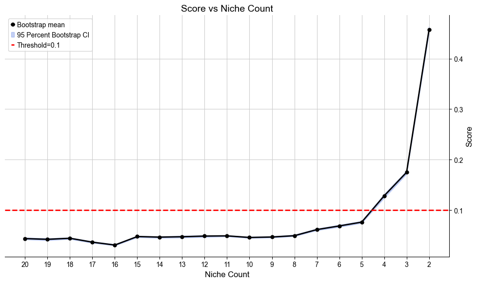
Done!
Perform overclustered initialization on the cell type distributions of cell neighborhoods for the case group. Resulting in Rmax new niches. The distributions of new niches are also computed.
[10]:
model.initialize_clusters_cond(assign_metric='jsd',  # default
                               threshold=0.1,  # default
                               min_cell_per_niche=100,  # default
                               dim_reduction=True,  # default
                               explained_var=None,  # default
                               n_components=None,  # default
                               n_components_max=100,  # default
                               standardize=True,  # default
                               method='kmeans',  # default
                               Rmax=10,  # default
                               )
Assigning cells to fixed niches...
11737 out of 1405182 cells are assigned to fixed niches.

Performing dimension reduction...
Returning 47 principal components.

Initializing niches...
10 new niches defined.
Perform hierarchical distribution matching for the case group to reduce the niche number to 0. This step results in niche assignment under a sequence of different niche numbers (usually from Rmax to 0).
[11]:
model.hier_dist_match_cond(assign_metric='jsd',  # default
                           weighted_merge=True,  # default
                           max_iters=100,  # default
                           tol=1e-4,  # default
                           )
Starting from 10 new cell niches...

Assigning cells to cell niche...
Current state: [0, 1, 2, 3, 4, 5, 6, 7, 8, 9, 10, 11, 12, 13]
22%|██▏ | 22/100 [01:15<04:28, 3.44s/it]
Distribution of cell niches (centers) converge at iteration 23.
10 new cell niches left.
Merging new cell niche 8 into basic cell niche 3...
Done!

Assigning cells to cell niche...
Current state: [0, 1, 2, 3, 4, 5, 6, 7, 9, 10, 11, 12, 13]
14%|█▍ | 14/100 [00:48<04:55, 3.44s/it]
Distribution of cell niches (centers) converge at iteration 15.
9 new cell niches left.
Merging new cell niche 12 into basic cell niche 2...
Done!

Assigning cells to cell niche...
Current state: [0, 1, 2, 3, 4, 5, 6, 7, 9, 10, 11, 13]
42%|████▏ | 42/100 [01:56<02:40, 2.77s/it]
Distribution of cell niches (centers) converge at iteration 43.
8 new cell niches left.
Merging new cell niche 13 into basic cell niche 2...
Done!

Assigning cells to cell niche...
Current state: [0, 1, 2, 3, 4, 5, 6, 7, 9, 10, 11]
29%|██▉ | 29/100 [01:22<03:21, 2.84s/it]
Distribution of cell niches (centers) converge at iteration 30.
7 new cell niches left.
Merging new cell niche 6 into basic cell niche 2...
Done!

Assigning cells to cell niche...
Current state: [0, 1, 2, 3, 4, 5, 7, 9, 10, 11]
11%|█ | 11/100 [00:27<03:39, 2.47s/it]
Distribution of cell niches (centers) converge at iteration 12.
6 new cell niches left.
Merging new cell niche 9 into basic cell niche 2...
Done!

Assigning cells to cell niche...
Current state: [0, 1, 2, 3, 4, 5, 7, 10, 11]
29%|██▉ | 29/100 [01:17<03:09, 2.66s/it]
Distribution of cell niches (centers) converge at iteration 30.
5 new cell niches left.
Merging new cell niche 5 into basic cell niche 2...
Done!

Assigning cells to cell niche...
Current state: [0, 1, 2, 3, 4, 7, 10, 11]
20%|██ | 20/100 [00:44<02:57, 2.21s/it]
Distribution of cell niches (centers) converge at iteration 21.
4 new cell niches left.
Merging new cell niche 7 into basic cell niche 2...
Done!

Assigning cells to cell niche...
Current state: [0, 1, 2, 3, 4, 10, 11]
19%|█▉ | 19/100 [00:36<02:36, 1.93s/it]
Distribution of cell niches (centers) converge at iteration 20.
3 new cell niches left.
Merging new cell niche 4 into basic cell niche 2...
Done!

Assigning cells to cell niche...
Current state: [0, 1, 2, 3, 10, 11]
22%|██▏ | 22/100 [00:46<02:46, 2.13s/it]
Distribution of cell niches (centers) converge at iteration 23.
2 new cell niches left.
Merging new cell niche 11 into basic cell niche 2...
Done!

Assigning cells to cell niche...
Current state: [0, 1, 2, 3, 10]
5%|▌ | 5/100 [00:09<02:58, 1.88s/it]
Distribution of cell niches (centers) converge at iteration 6.
1 new cell niches left.
Merging new cell niche 10 into basic cell niche 0...
Done!

Assigning cells to cell niche...
Current state: [0, 1, 2, 3]
No new cell niche, all cells assigned to basic niches.
0 new cell niches left.
No new cell niche left.

Finished!
Automatically define the most appropriate number of condition-specific niches based on minJSD score for the case group. The results of niche assignments are saved in .obs[niche_key] and .obs[csn_label]. All basic cell niches are named “basic” in .obs[csn_label] and condition-specific niches start with a prefix “R”.
[12]:
cond_list, cond_concat = model.select_solution_cond(n_csn=None,  # default
                                                    niche_key='niche_label',  # default
                                                    csn_key='csn_label',  # default
                                                    auto=True,  # default
                                                    metric='jsd_v2',  # default
                                                    threshold=0.1,  # default
                                                    return_adata=True,  # default
                                                    plot=True,  # default
                                                    save=False,  # default
                                                    fig_size=(10, 6),  # default
                                                    save_dir=save_dir,
                                                    file_name='score_vs_nichecount_cond.pdf',
                                                    )
Automatically selecting best solution...
100%|██████████| 100/100 [00:09<00:00, 10.29it/s]
100%|██████████| 100/100 [00:09<00:00, 10.37it/s]
100%|██████████| 100/100 [00:09<00:00, 10.59it/s]
100%|██████████| 100/100 [00:08<00:00, 12.07it/s]
100%|██████████| 100/100 [00:07<00:00, 13.26it/s]
100%|██████████| 100/100 [00:06<00:00, 14.48it/s]
100%|██████████| 100/100 [00:05<00:00, 17.12it/s]
100%|██████████| 100/100 [00:05<00:00, 18.92it/s]
100%|██████████| 100/100 [00:04<00:00, 21.44it/s]
100%|██████████| 100/100 [00:01<00:00, 91.19it/s]
Suggested range of condition specific niche count is from 3 to 4.
Recommended number of condition specific niches are [4]
Selecting 4 new niches as the best solution.
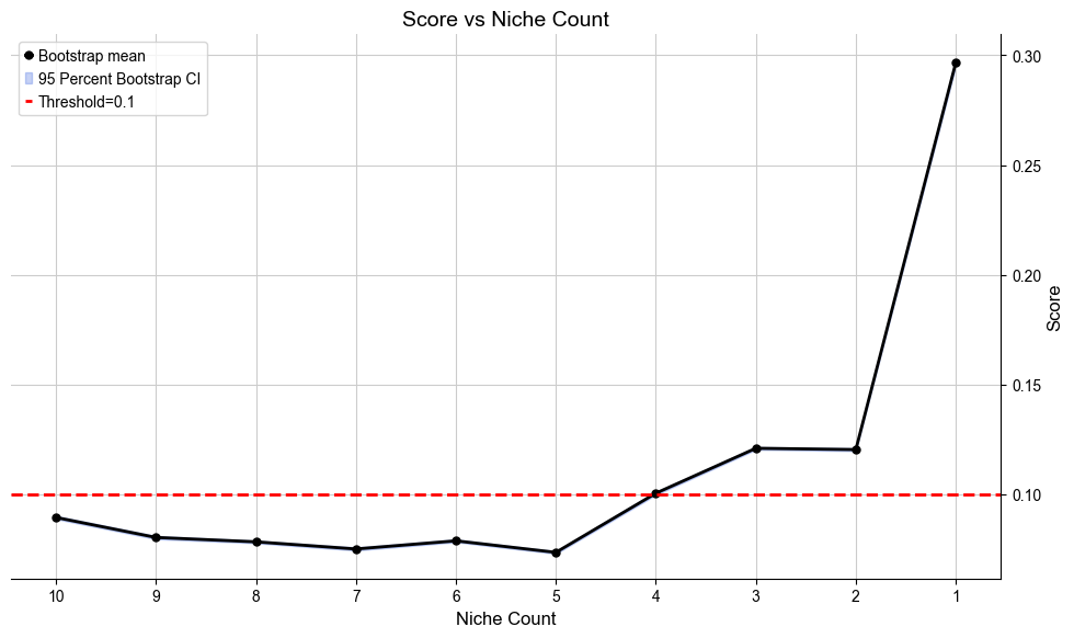
Done!
Save results
[ ]:
ctr_concat.write_h5ad(save_dir + 'Harmonics_basic_result_0.h5ad')
cond_concat.write_h5ad(save_dir + 'Harmonics_cond_result_0.h5ad')
Save and reload the results. Normalize the data for downstream analysis.
[7]:
ctr_concat = ad.read_h5ad(save_dir + 'Harmonics_basic_result_0.h5ad')
cond_concat = ad.read_h5ad(save_dir + 'Harmonics_cond_result_0.h5ad')

for i, slice_name in enumerate(ctr_name_list):
    adata = ctr_concat[ctr_concat.obs['slice_name'] == slice_name, :].copy()
    sc.pp.normalize_total(adata, target_sum=1e4)
    sc.pp.log1p(adata)
    ctr_list[i] = adata
for i, slice_name in enumerate(cond_name_list):
    adata = cond_concat[cond_concat.obs['slice_name'] == slice_name, :].copy()
    sc.pp.normalize_total(adata, target_sum=1e4)
    sc.pp.log1p(adata)
    cond_list[i] = adata
[8]:
ctr_concat_new = ctr_concat.copy()
cond_concat_new = cond_concat.copy()
ctr_concat_new, cond_concat_new
[8]:
(AnnData object with n_obs × n_vars = 199773 × 343
     obs: 'sample', 'patient', 'cell_id', 'full_cell_id', 'sample_type', 'sample_affect', 'disease_status', 'percent_pathology', 'tma', 'run', 'final_CT', 'final_lineage', 'CNiche', 'TNiche', 'lumen_id', 'lumen_rank', 'x_centroid', 'y_centroid', 'adj_x_centroid', 'adj_y_centroid', 'super_adj_x_centroid', 'super_adj_y_centroid', 'nCount_RNA', 'nFeature_RNA', 'perc_negcontrolprobe', 'perc_negcontrolcodeword', 'perc_unassigned', 'perc_negcontrolorunassigned', 'slice_name', 'celltype_idx', 'n_neighbors', 'niche_label_20', 'niche_label_19', 'niche_label_18', 'niche_label_17', 'niche_label_16', 'niche_label_15', 'niche_label_14', 'niche_label_13', 'niche_label_12', 'niche_label_11', 'niche_label_10', 'niche_label_9', 'niche_label_8', 'niche_label_7', 'niche_label_6', 'niche_label_5', 'niche_label_4', 'niche_label_3', 'niche_label_2', 'niche_label_jsd_v2', 'niche_label_jsd', 'niche_label_fmi', 'niche_label_ari', 'niche_label_nmi', 'niche_label_asw', 'niche_label_js_asw', 'niche_label_fisher', 'niche_label_chi', 'niche_label_dbi', 'niche_label_dass_mean', 'niche_label_dass_min', 'niche_label_dafisher', 'niche_label_dachi', 'niche_label_0.09', 'niche_label_0.11', 'niche_label'
     uns: 'ct2idx', 'idx2ct', 'niche_cell_count', 'niche_dist', 'niche_label_summary', 'score_dict'
     obsm: 'micro_dist', 'onehot', 'spatial',
 AnnData object with n_obs × n_vars = 1405182 × 343
     obs: 'sample', 'patient', 'cell_id', 'full_cell_id', 'sample_type', 'sample_affect', 'disease_status', 'percent_pathology', 'tma', 'run', 'final_CT', 'final_lineage', 'CNiche', 'TNiche', 'lumen_id', 'lumen_rank', 'x_centroid', 'y_centroid', 'adj_x_centroid', 'adj_y_centroid', 'super_adj_x_centroid', 'super_adj_y_centroid', 'nCount_RNA', 'nFeature_RNA', 'perc_negcontrolprobe', 'perc_negcontrolcodeword', 'perc_unassigned', 'perc_negcontrolorunassigned', 'slice_name', 'celltype_idx', 'n_neighbors', 'niche_label_10', 'csn_label_10', 'niche_label_9', 'csn_label_9', 'niche_label_8', 'csn_label_8', 'niche_label_7', 'csn_label_7', 'niche_label_6', 'csn_label_6', 'niche_label_5', 'csn_label_5', 'niche_label_4', 'csn_label_4', 'niche_label_3', 'csn_label_3', 'niche_label_2', 'csn_label_2', 'niche_label_1', 'csn_label_1', 'niche_label_0', 'csn_label_0', 'niche_label_jsd_v2', 'csn_label_jsd_v2', 'niche_label_jsd', 'csn_label_jsd', 'niche_label_fmi', 'csn_label_fmi', 'niche_label_ari', 'csn_label_ari', 'niche_label_nmi', 'csn_label_nmi', 'niche_label_asw', 'csn_label_asw', 'niche_label_js_asw', 'csn_label_js_asw', 'niche_label_fisher', 'csn_label_fisher', 'niche_label_chi', 'csn_label_chi', 'niche_label_dbi', 'csn_label_dbi', 'niche_label_dass_mean', 'csn_label_dass_mean', 'niche_label_dass_min', 'csn_label_dass_min', 'niche_label_dafisher', 'csn_label_dafisher', 'niche_label_dachi', 'csn_label_dachi', 'niche_label_0.09', 'csn_label_0.09', 'niche_label_0.11', 'csn_label_0.11', 'niche_label', 'csn_label'
     uns: 'ct2idx', 'idx2ct', 'niche_cell_count', 'niche_dist', 'niche_label_summary', 'score_dict'
     obsm: 'micro_dist', 'onehot', 'spatial')
Plot the results
[9]:
niches = cond_concat_new.uns['niche_label_summary']
niche_colors = ['#1f77b4', '#ff7f0e', '#279e68', '#d62728', '#aa40fc', '#e377c2', '#8c564b', '#b5bd61',]
# niche_colors = ['#1f77b4', '#ff7f0e', '#279e68', '#d62728', '#aa40fc', '#8c564b', '#e377c2', '#b5bd61', '#17becf',
#                 '#aec7e8', '#ffbb78', '#98df8a', '#ff9896', '#c5b0d5', '#c49c94', '#f7b6d2', '#dbdb8d', '#9edae5']
niche_color_dict = {niches[k]: niche_colors[k] for k in range(len(niches))}

n_basic_niches = len(ctr_concat.uns['niche_label_summary'])
csns = [f'R{int(label)-n_basic_niches}' for label in niches[n_basic_niches:]]
csn_color_dict = {csns[k]: niche_colors[k+n_basic_niches] for k in range(len(csns))}
csn_color_dict['basic'] = '#d3d3d3'

celltypes = ['AT1', 'AT2', 'Activated Fibrotic FBs', 'Adventitial FBs', 'Alveolar FBs', 'Alveolar Macrophages', 'Arteriole', 'B cells',
             'Basal', 'Basophils', 'CD4+ T-cells', 'CD8+ T-cells', 'Capillary', 'Goblet', 'Inflammatory FBs', 'Interstitial Macrophages',
             'KRT5-/KRT17+', 'Langerhans cells', 'Lymphatic', 'Macrophages - IFN-activated', 'Mast', 'Mesothelial', 'Migratory DCs',
             'Monocytes/MDMs', 'Multiciliated', 'Myofibroblasts', 'NK/NKT', 'Neutrophils', 'PNEC', 'Plasma', 'Proliferating AT2',
             'Proliferating Airway', 'Proliferating B cells', 'Proliferating FBs', 'Proliferating Myeloid', 'Proliferating NK/NKT',
             'Proliferating T-cells', 'RASC', 'SMCs/Pericytes', 'SPP1+ Macrophages', 'Secretory', 'Subpleural FBs', 'Transitional AT2',
             'Tregs', 'Venous', 'cDCs', 'pDCs']
ct_colors = ['#ffff00', '#1ce6ff', '#ff34ff', '#00846f', '#008941', '#00c2a0', '#a30059', '#4fc601',
             '#d16100', '#c2ffed', '#63ffac', '#0000a6', '#b79762', '#004d43', '#006fa6', '#997d87',
             '#a079bf', '#ddefff', '#809693', '#1b4400', '#3b5dff', '#cc0744', '#ff2f80',
             '#61615a', '#ba0900', '#6b7900', '#ffdbe5', '#ffaa92', '#ff90c9', '#b903aa', '#4a3b53',
             '#5a0007', '#000035', '#7b4f4b', '#372101', '#300018',
             '#7a4900', '#013349', '#ff4a46', '#ffb500', '#8fb0ff', '#0aa6d8', "#74926C",
             '#c2ff99', '#c0b9b2', '#001e09', '#6a3a4c',]
ct_color_dict = {ct: color for ct, color in zip(celltypes, ct_colors)}
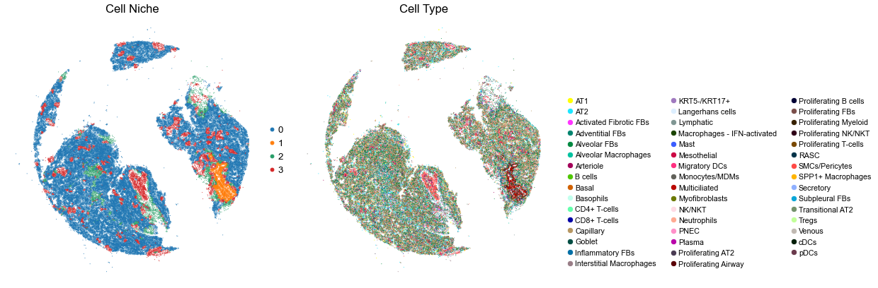
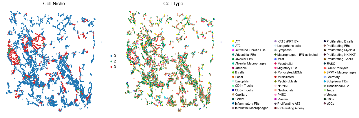
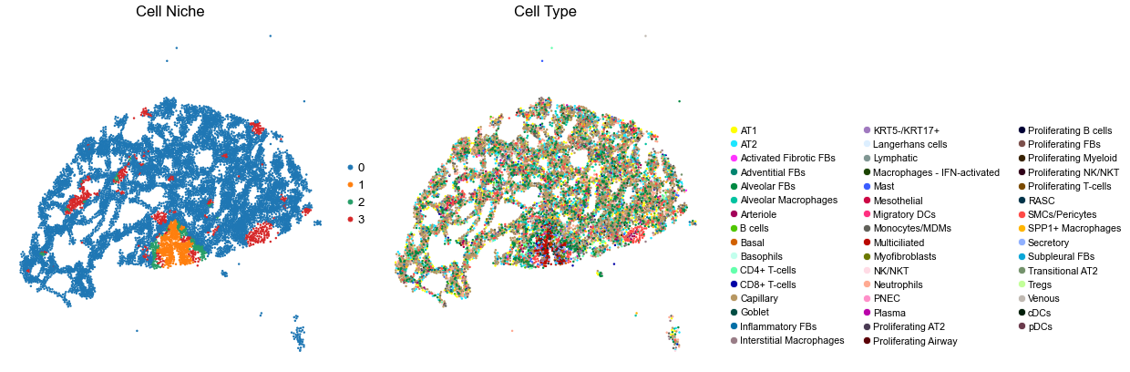
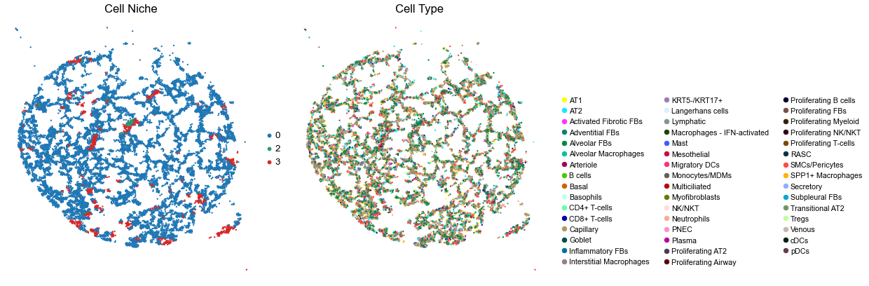
Control group
[10]:
for i in range(len(ctr_name_list)):

    print(ctr_name_list[i])
    adata = ctr_concat_new[ctr_concat_new.obs['slice_name'] == ctr_name_list[i], :].copy()
    n_cell = adata.shape[0]
    print(n_cell)
    print(adata.obs['percent_pathology'][0])
    s = 4e5 / n_cell

    fig, axes = plt.subplots(1, 2, figsize=(21, 7))

    sc.pl.embedding(adata, basis='spatial', color='niche_label', palette=niche_color_dict,
                    ax=axes[0], s=s, show=False, frameon=False, title='Cell Niche', legend_fontsize=16)
    axes[0].set_title('Cell Niche', fontsize=20)
    axes[0].invert_yaxis()

    sc.pl.embedding(adata, basis='spatial', color='final_CT', palette=ct_color_dict,
                    ax=axes[1], s=s, show=False, frameon=False, title='Cell Type', legend_fontsize=16)
    axes[1].set_title('Cell Type', fontsize=20)
    axes[1].invert_yaxis()

    ct_legend_elements = [
        Line2D([0], [0], marker='o', color='w', label=label,
            markerfacecolor=color, markersize=10)
        for label, color in ct_color_dict.items()
    ]
    axes[1].legend(handles=ct_legend_elements, loc=(1.05, 0.05), frameon=False, ncol=3)
    axes[1].axis('off')

    plt.tight_layout()
    plt.show()
THD0008
69227
0.0
VUHD038
5941
5.0
VUHD049
22688
0.0
VUHD069
19976
0.0
VUHD090
16110
5.0
VUHD095
11442
0.0
VUHD113
12870
0.0
VUHD116A
12372
0.0
VUHD116B
29147
0.0
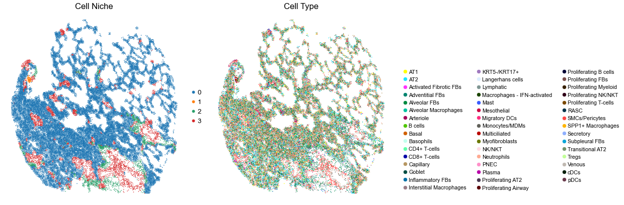
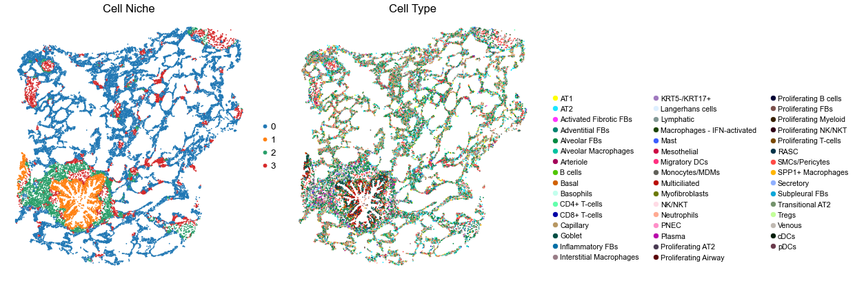
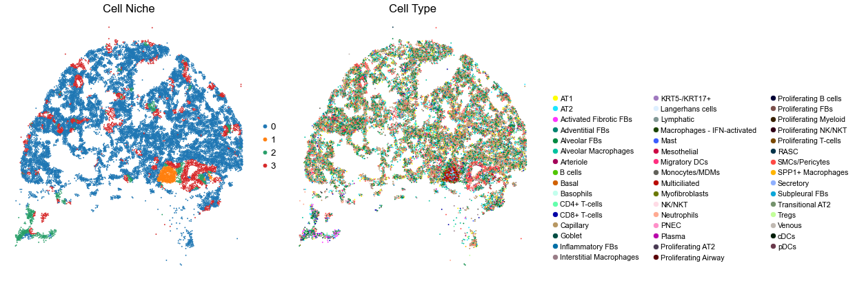
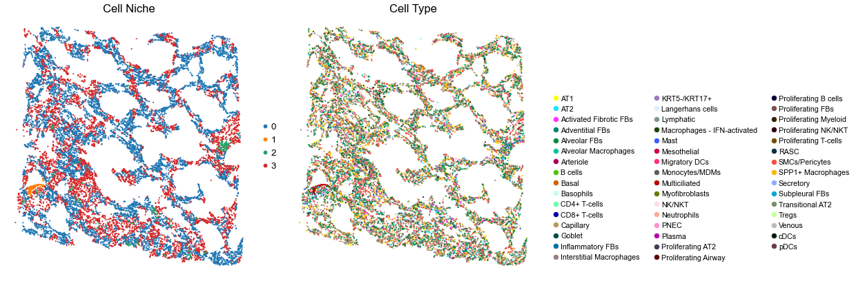
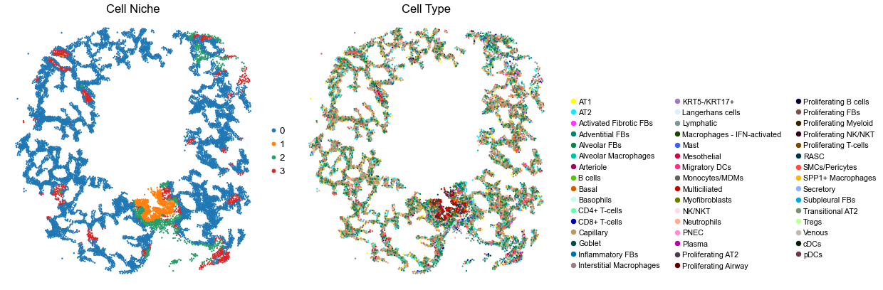
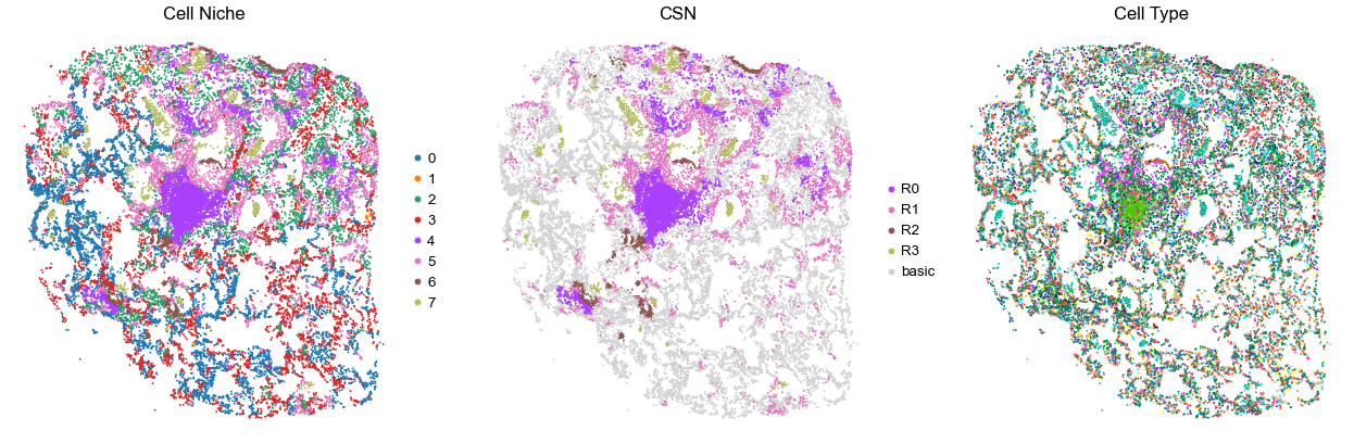
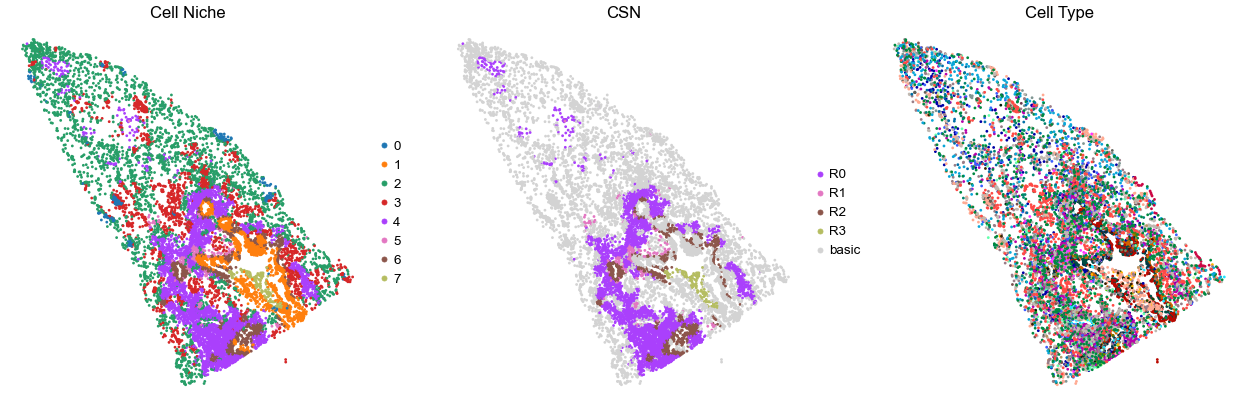
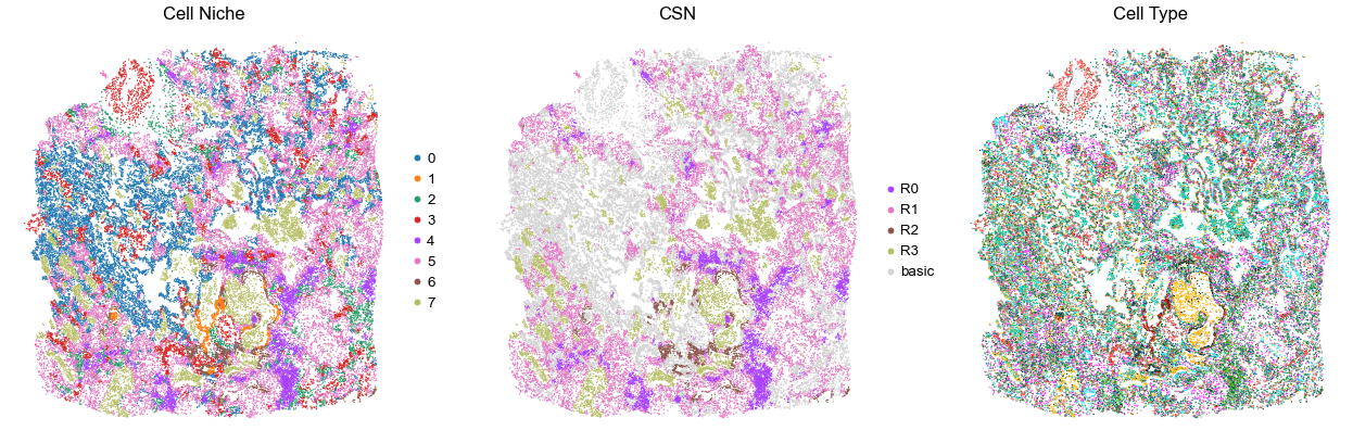
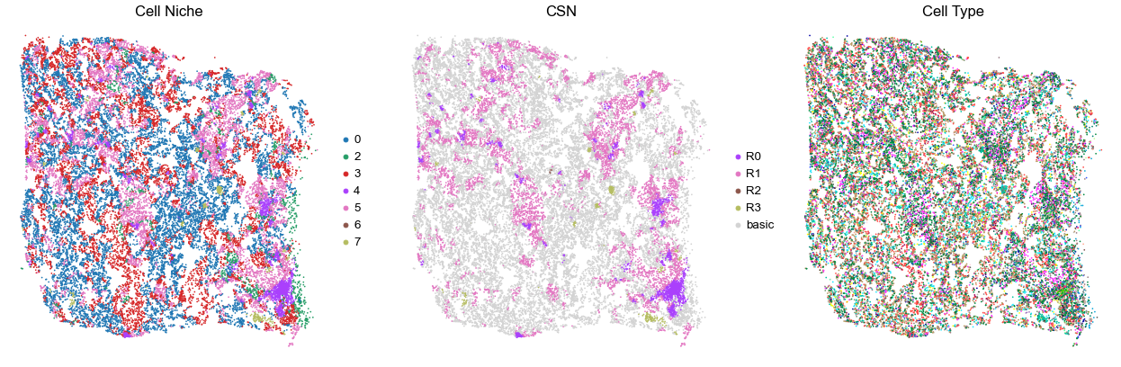
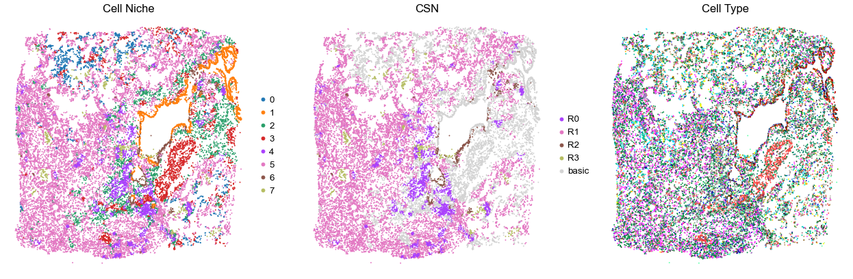
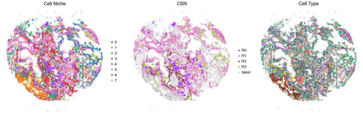
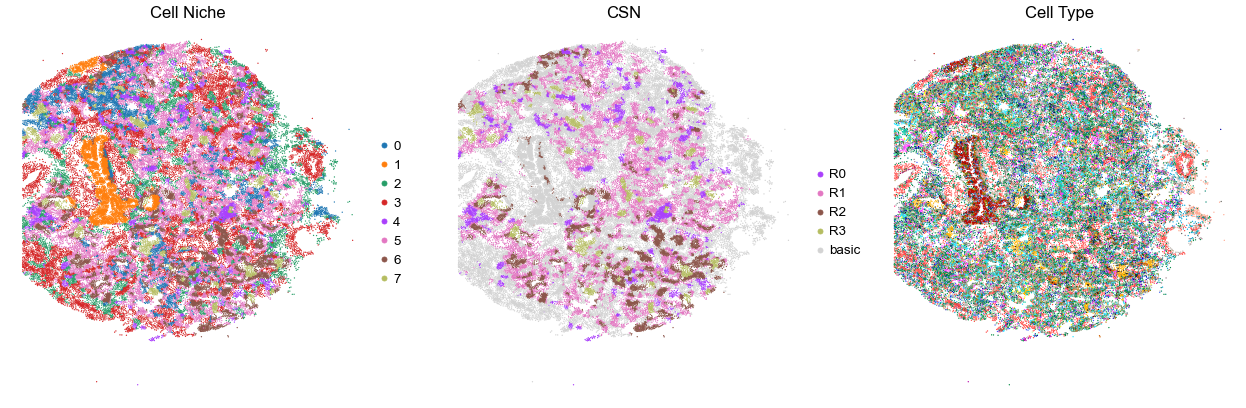
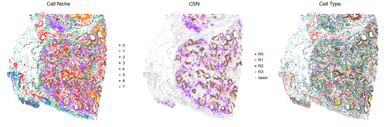
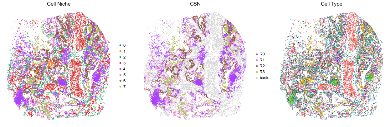
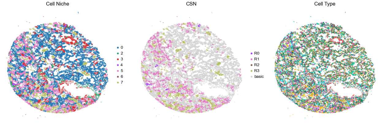
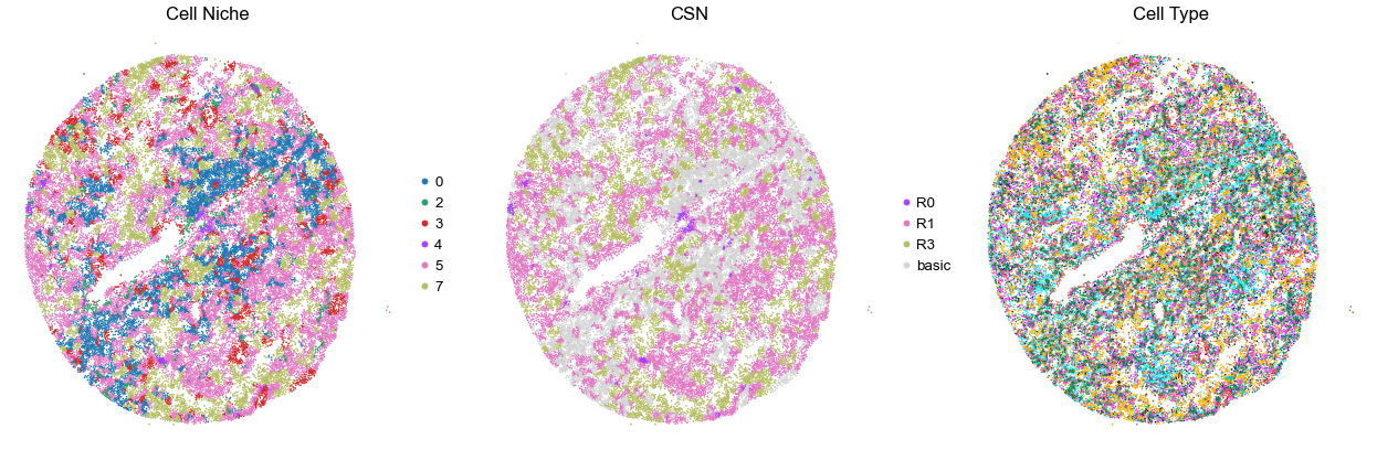
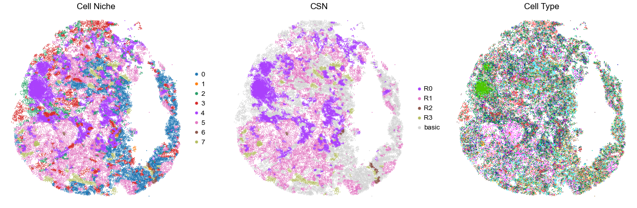
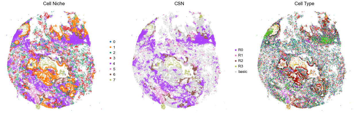
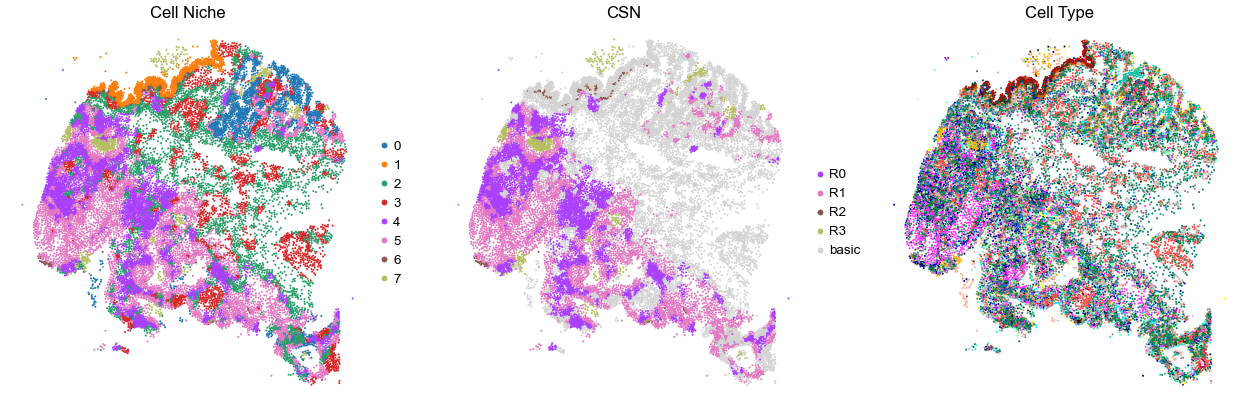
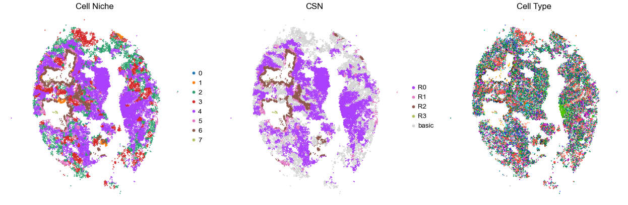
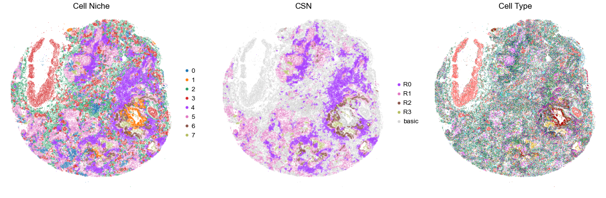
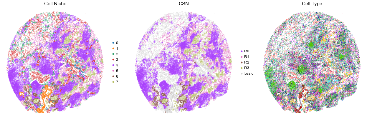
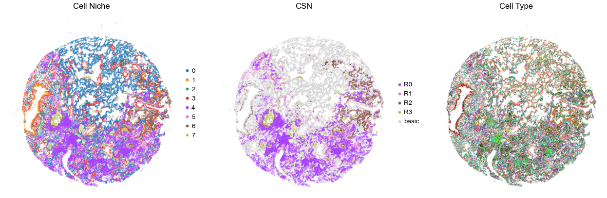
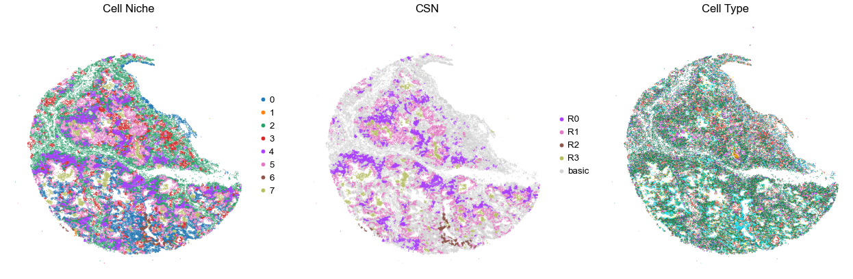
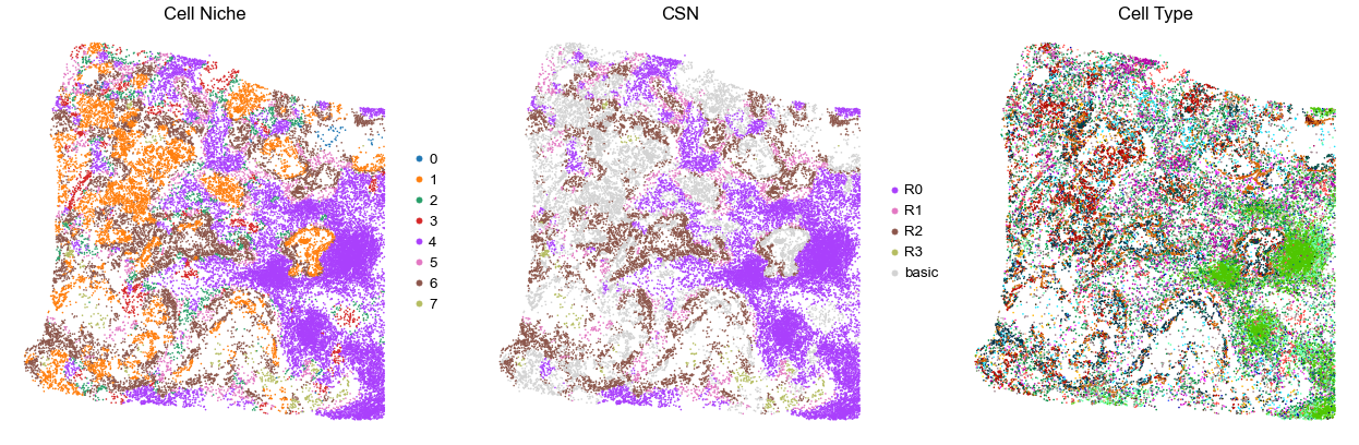
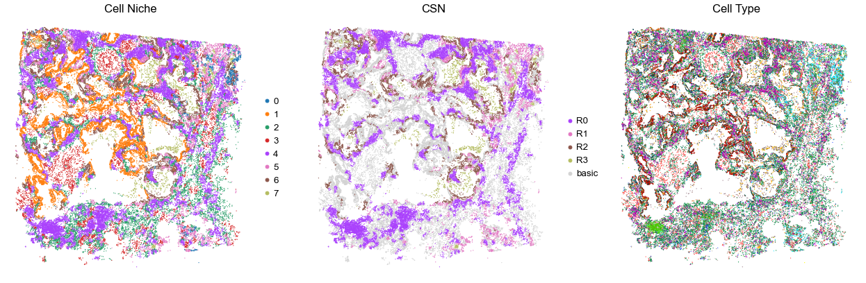
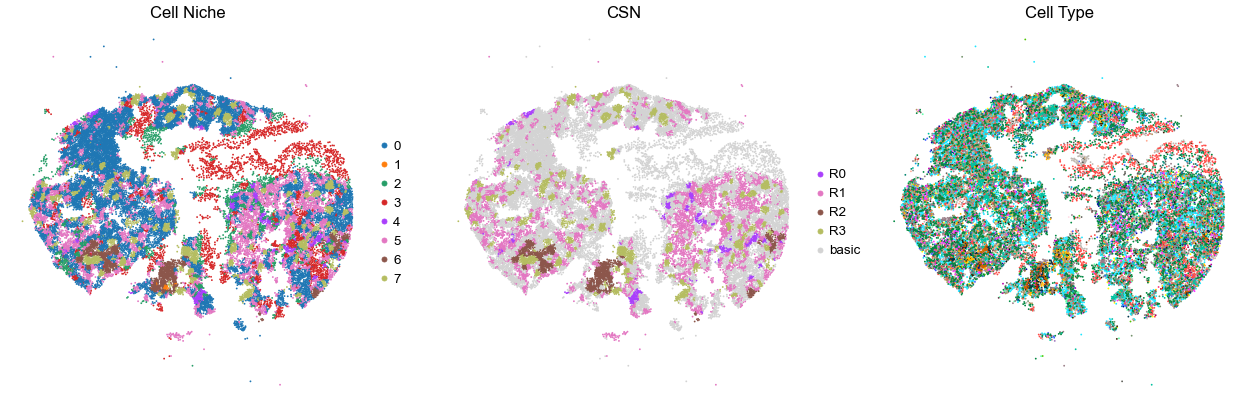
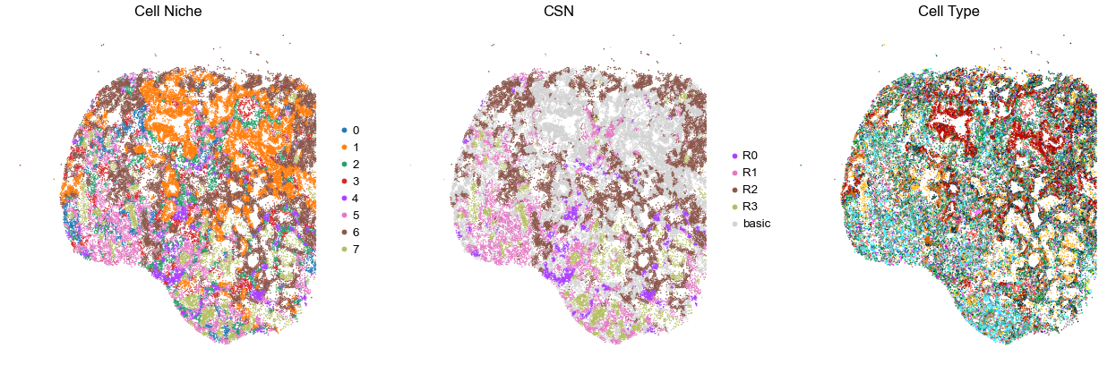
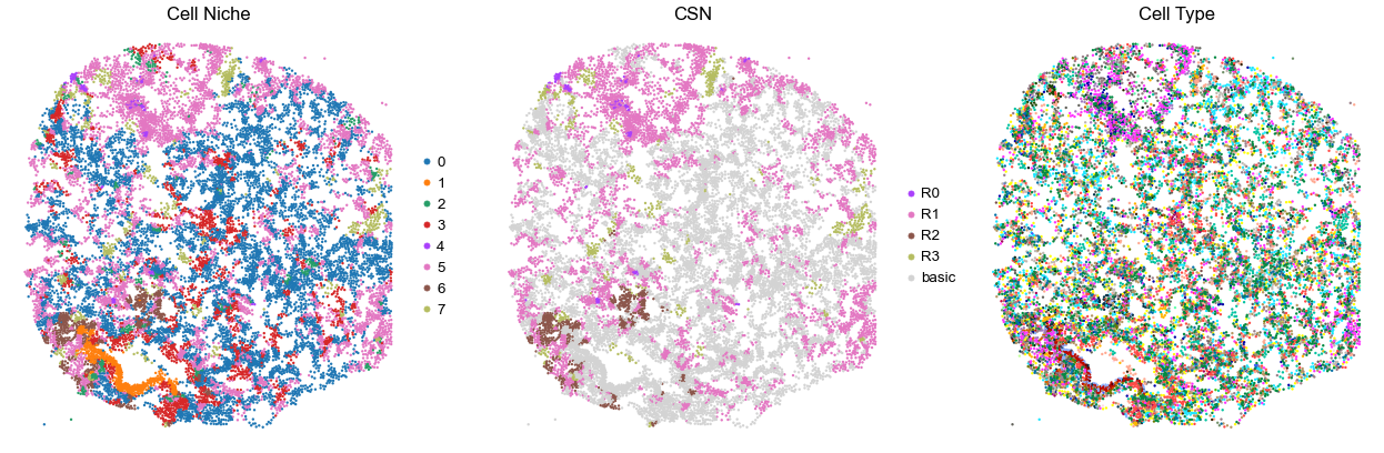
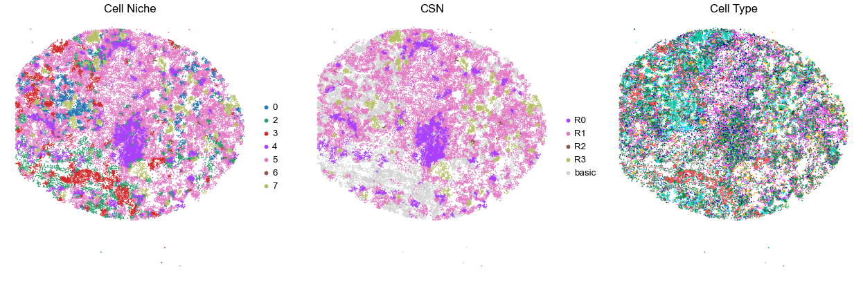
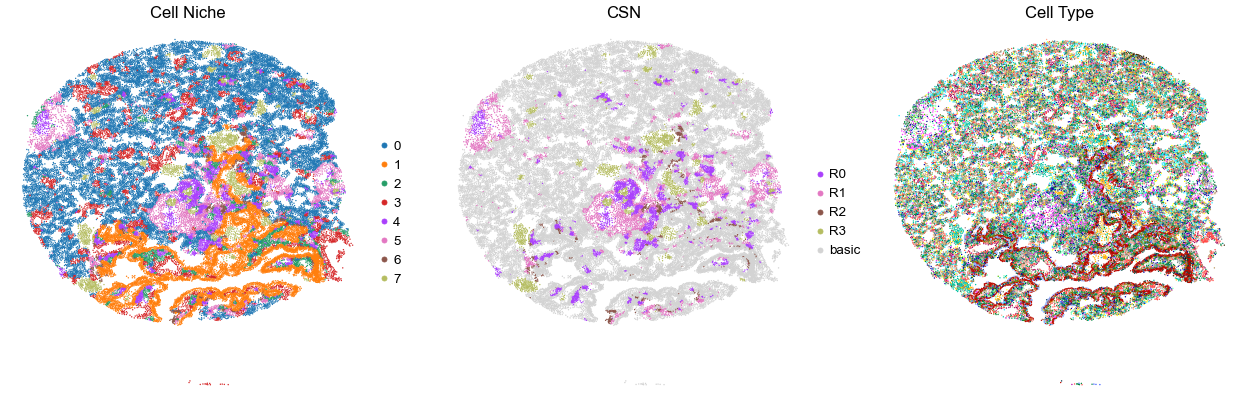
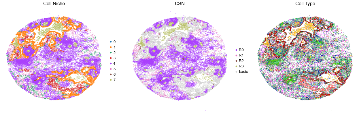
Case group
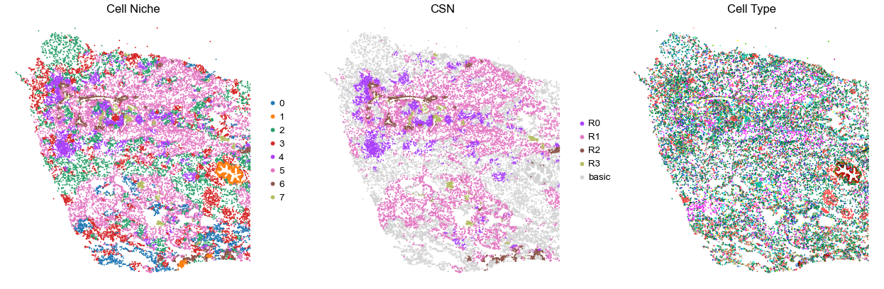
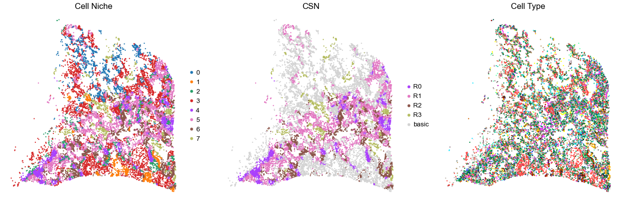
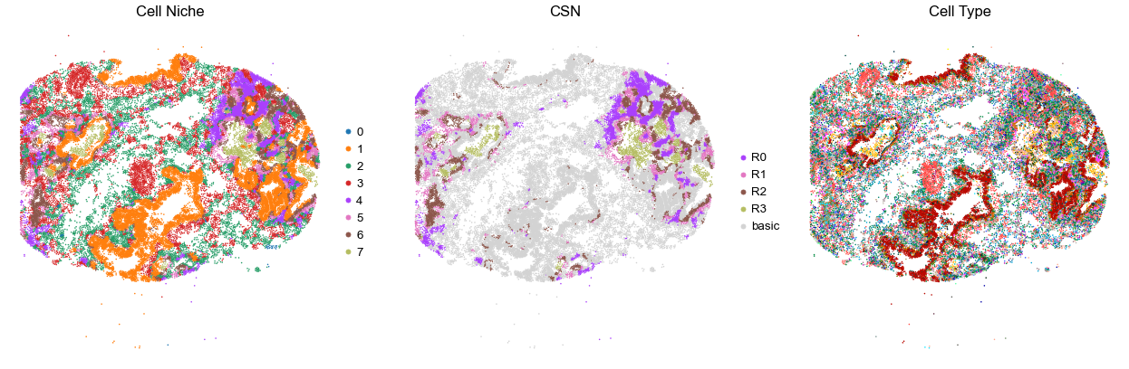
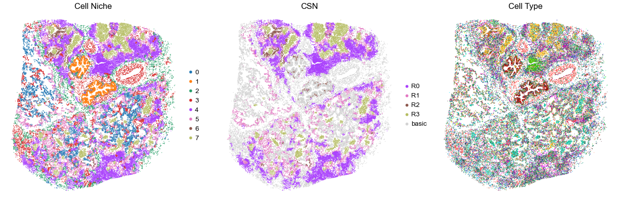
[11]:
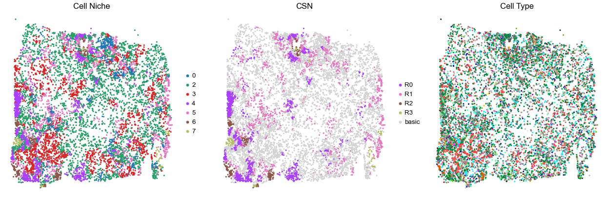
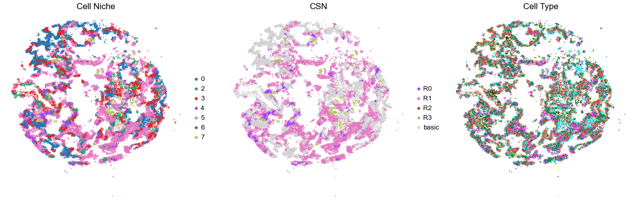
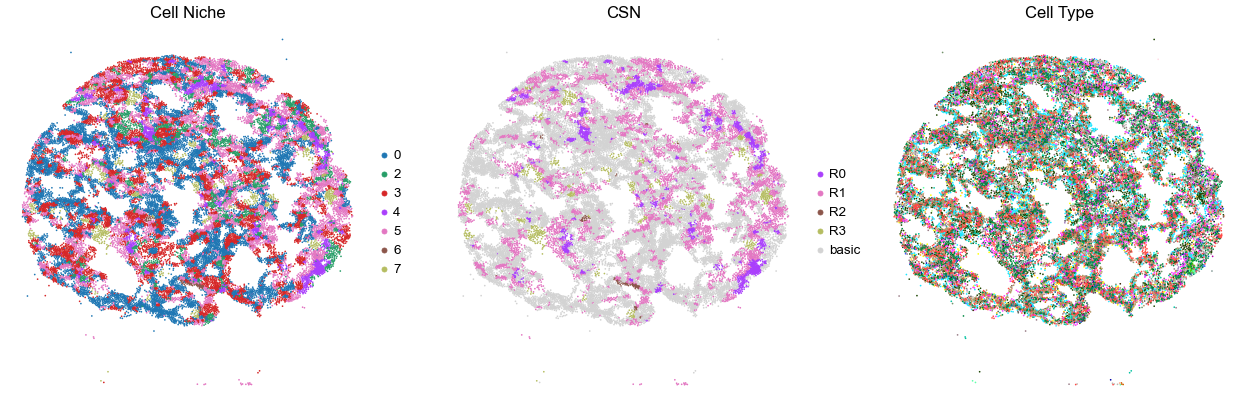
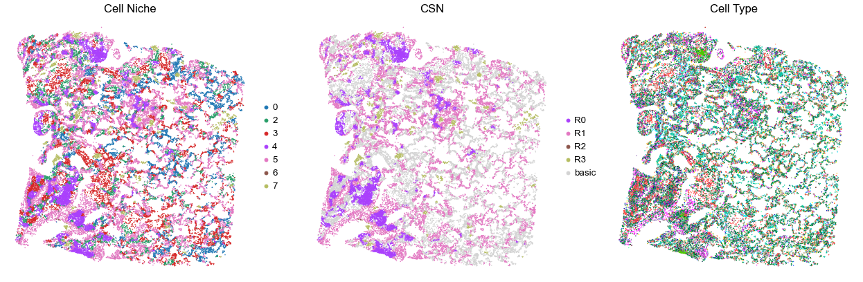
for i in range(len(cond_name_list)):

    print(cond_name_list[i])
    adata = cond_concat_new[cond_concat_new.obs['slice_name'] == cond_name_list[i], :].copy()
    n_cell = adata.shape[0]
    print(adata.obs['tma'][0])
    print(n_cell)
    print(adata.obs['percent_pathology'][0])
    s = 5e5 / n_cell

    fig, axes = plt.subplots(1, 3, figsize=(21, 7))

    sc.pl.embedding(adata, basis='spatial', color='niche_label', palette=niche_color_dict,
                    ax=axes[0], s=s, show=False, frameon=False, title='Cell Niche', legend_fontsize=16)
    axes[0].set_title('Cell Niche', fontsize=20)
    axes[0].invert_yaxis()

    sc.pl.embedding(adata, basis='spatial', color='csn_label', palette=csn_color_dict,
                    ax=axes[1], s=s, show=False, frameon=False, title='CSN', legend_fontsize=16)
    axes[1].set_title('CSN', fontsize=20)
    axes[1].invert_yaxis()

    sc.pl.embedding(adata, basis='spatial', color='final_CT', palette=ct_color_dict,
                    ax=axes[2], s=s, show=False, frameon=False, title='Cell Type', legend_loc=None)
    axes[2].set_title('Cell Type', fontsize=20)
    axes[2].invert_yaxis()

    plt.tight_layout()
    plt.show()
TILD028LA
TMA5
24813
45.0
TILD049MA
TMA5
11140
100.0
TILD080LA
TMA5
51212
65.0
TILD111LA
TMA5
29566
20.0
TILD113LA
TMA5
24202
55.0
TILD117LA
TMA4
36707
50.0
TILD117MA1
TMA4
49231
95.0
TILD117MA2
TMA5
35271
90.0
TILD130LA
TMA5
24547
70.0
TILD167LA
TMA5
15870
50.0
TILD175MA
TMA4
35887
95.0
TILD299MA
TMA5
52992
75.0
TILD315MA
TMA5
37361
100.0
VUILD102LA
TMA1
26364
35.0
VUILD102MA
TMA1
31517
95.0
VUILD104MA1
TMA2
35502
85.0
VUILD104MA2
TMA2
37764
90.0
VUILD105MA1
TMA2
21108
90.0
VUILD105MA2
TMA2
21178
95.0
VUILD106MA
TMA3
124717
100.0
VUILD107MA
TMA1
68413
100.0
VUILD110LA
TMA3
122815
55.0
VUILD115MA
TMA3
94540
100.0
VUILD141MA
TMA5
34702
100.0
VUILD142MA
TMA5
9222
95.0
VUILD48LA1
TMA2
20819
20.0
VUILD48LA2
TMA2
30302
40.0
VUILD49LA
TMA5
38280
45.0
VUILD58MA
TMA5
56733
100.0
VUILD78LA
TMA4
26235
65.0
VUILD78MA
TMA4
35306
85.0
VUILD91LA
TMA4
15468
15.0
VUILD91MA
TMA4
24553
75.0
VUILD96LA
TMA1
44367
30.0
VUILD96MA
TMA1
56478
100.0
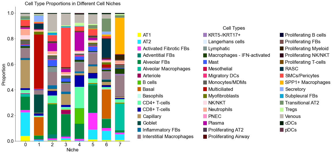
Cell type composition (control group)
[12]:
basic_niche_labels = ctr_concat_new.uns['niche_label_summary'].copy()
ct_labels = sorted(cond_concat_new.obs['final_CT'].unique())
basic_niche_dist = ctr_concat_new.uns['niche_dist'].toarray().copy()
basic_cell_count_niche = ctr_concat_new.uns['niche_cell_count'].copy()

fig, ax = plt.subplots(figsize=(5, 9))
bar_width = 0.7
n_niches, n_cell_types = basic_niche_dist.shape

x = np.arange(n_niches)

for j in range(n_cell_types):
    bottom = np.sum(basic_niche_dist[:, :j], axis=1)
    ax.bar(x,
           basic_niche_dist[:, j],
           bottom=bottom,
           width=bar_width,
           color=ct_color_dict[ct_labels[j]],
           label=ct_labels[j])

ax.set_ylabel('Proportion', fontsize=20)
ax.set_xlabel('Niche', fontsize=20)
ax.set_xticks(x)
ax.set_xticklabels(basic_niche_labels, rotation=0, ha='center')
ax.tick_params(axis='x', labelsize=20)
ax.tick_params(axis='y', labelsize=20)
ax.spines['top'].set_visible(False)
ax.spines['right'].set_visible(False)
ax.grid(False)

handles = [
    mpatches.Patch(color=color, label=ct)
    for ct, color in zip(celltypes, ct_colors)
]

ax.legend(handles=handles, title='Cell Types', loc=(1.05, 0.0), frameon=False, handleheight=0.8,
          handlelength=0.7, ncol=3, fontsize=20, title_fontsize=20)

plt.title('Cell Type Proportions in Different Cell Niches', fontsize=20)
plt.tight_layout()
plt.show()
Cell type composition (case group)
[13]:
cond_niche_labels = cond_concat_new.uns['niche_label_summary'].copy()
ct_labels = sorted(cond_concat_new.obs['final_CT'].unique())
cond_niche_dist = cond_concat_new.uns['niche_dist'].toarray().copy()
cond_cell_count_niche = cond_concat_new.uns['niche_cell_count'].copy()

fig, ax = plt.subplots(figsize=(20, 9))
bar_width = 0.7
n_niches, n_cell_types = cond_niche_dist.shape

x = np.arange(n_niches)

for j in range(n_cell_types):
    bottom = np.sum(cond_niche_dist[:, :j], axis=1)
    ax.bar(x,
           cond_niche_dist[:, j],
           bottom=bottom,
           width=bar_width,
           color=ct_color_dict[ct_labels[j]],
           label=ct_labels[j])

ax.set_ylabel('Proportion', fontsize=20)
ax.set_xlabel('Niche', fontsize=20)
ax.set_xticks(x)
ax.set_xticklabels(cond_niche_labels, rotation=0, ha='center')
ax.tick_params(axis='x', labelsize=20)
ax.tick_params(axis='y', labelsize=20)
ax.spines['top'].set_visible(False)
ax.spines['right'].set_visible(False)
ax.grid(False)

handles = [
    mpatches.Patch(color=color, label=ct)
    for ct, color in zip(celltypes, ct_colors)
]

ax.legend(handles=handles, title='Cell Types', loc=(1.05, 0.0), frameon=False, handleheight=0.8,
          handlelength=0.7, ncol=3, fontsize=20, title_fontsize=20)

plt.title('Cell Type Proportions in Different Cell Niches', fontsize=20)
plt.tight_layout()
plt.show()
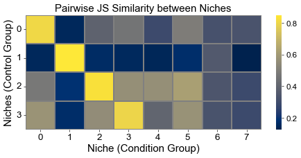
Calculate the similarity between niches from different groups
Similarities are measured using 1-JSD score
[14]:
from scipy.spatial.distance import jensenshannon
from scipy.stats import pearsonr
from sklearn.metrics.pairwise import cosine_similarity

basic_niche_dist = ctr_concat_new.uns['niche_dist'].toarray().copy()
cond_niche_dist = cond_concat_new.uns['niche_dist'].toarray().copy()

basic_niche_labels = ctr_concat_new.uns['niche_label_summary'].copy()
cond_niche_labels = cond_concat_new.uns['niche_label_summary'].copy()

n_niche_basic = basic_niche_dist.shape[0]
n_niche_cond = cond_niche_dist.shape[0]

js_sim = np.zeros((n_niche_basic, n_niche_cond))
# cos_sim = cosine_similarity(basic_niche_dist, cond_niche_dist)
# corr_sim = np.zeros((n_niche_basic, n_niche_cond))

for i in range(n_niche_basic):
    for j in range(n_niche_cond):
        js_sim[i, j] = 1 - jensenshannon(basic_niche_dist[i], cond_niche_dist[j], base=2)
        # corr_sim[i, j], _ = pearsonr(basic_niche_dist[i], cond_niche_dist[j])

plt.figure(figsize=(8, 4))
sns.heatmap(
    js_sim,
    cmap='cividis',
    xticklabels=cond_niche_labels,
    yticklabels=basic_niche_labels,
    linewidths=0.5,
    linecolor='gray',
)
plt.xlabel("Niche (Condition Group)", fontsize=18)
plt.ylabel("Niches (Control Group)", fontsize=18)
plt.title("Pairwise JS Similarity between Niches", fontsize=18)
plt.xticks(fontsize=16, rotation=0)
plt.yticks(fontsize=16, rotation=0)
plt.grid(False)
plt.tight_layout()
plt.show()
Cell type enrichment analysis
[15]:
ct_df = ct_enrichment_test(cond_concat_new.uns['niche_dist'],
                           cond_concat_new.uns['niche_cell_count'],
                           cond_concat_new.uns['idx2ct'],
                           cond_concat_new.uns['niche_label_summary'],
                           method='fisher',
                           alpha=0.05,
                           fdr_method='fdr_by',
                           log2fc_threshold=1,
                           prop_threshold=0.01,
                           verbose=True,
                           )
ct_df.head()
8 niches and 47 cell types in total.
[15]:
| niche_idx | niche | celltype_idx | celltype | oddsratio | p-value | q-value | log2fc | prop | enrichment | |
|---|---|---|---|---|---|---|---|---|---|---|
| 0 | 0 | 0 | 0 | AT1 | 8.188377 | 0.0 | 0.0 | 2.982605 | 0.039544 | True |
| 1 | 0 | 0 | 1 | AT2 | 7.536809 | 0.0 | 0.0 | 2.660621 | 0.185680 | True |
| 2 | 0 | 0 | 2 | Activated Fibrotic FBs | 0.439605 | 0.0 | 0.0 | -1.154935 | 0.016920 | False |
| 3 | 0 | 0 | 3 | Adventitial FBs | 0.108820 | 0.0 | 0.0 | -3.191124 | 0.000752 | False |
| 4 | 0 | 0 | 4 | Alveolar FBs | 0.670380 | 0.0 | 0.0 | -0.505470 | 0.103303 | False |
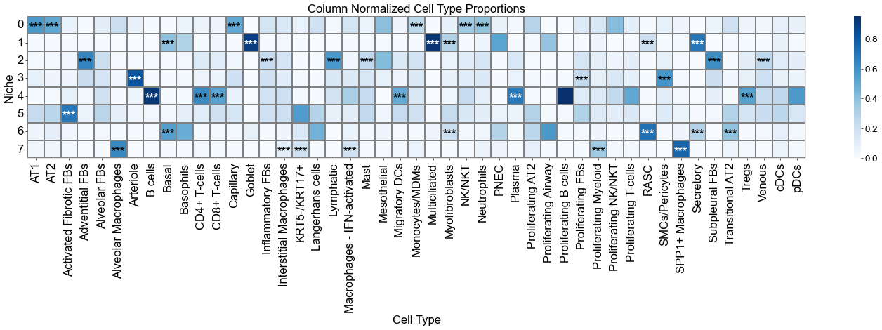
[16]:
niche_labels = cond_concat_new.uns['niche_label_summary'].copy()
ct_labels = sorted(cond_concat_new.obs['final_CT'].unique())

matrix_df = pd.DataFrame(
    data=cond_concat_new.uns['niche_dist'].toarray(),
    index=niche_labels,
    columns=ct_labels,
)

cn_dist_count = cond_concat_new.uns['niche_dist'].toarray() * cond_concat_new.uns['niche_cell_count'][:, np.newaxis]
cn_dist_norm = cn_dist_count / np.sum(cn_dist_count, axis=0)
matrix_df_norm = pd.DataFrame(
    data=cn_dist_norm,
    index=niche_labels,
    columns=ct_labels,
)

ct_df['stars'] = ct_df['q-value'].apply(p2stars)

stars_df = pd.DataFrame(
    '',
    index=matrix_df.index,
    columns=matrix_df.columns
)

for _, row in ct_df[ct_df['enrichment']].iterrows():
    niche = row['niche']
    ct    = row['celltype']
    if (niche in stars_df.index) and (ct in stars_df.columns):
        stars_df.loc[niche, ct] = row['stars']


fig, axes = plt.subplots(1, 1, figsize=(24, 8))

sns_heatmap_0 = sns.heatmap(
    matrix_df,
    cmap='Blues',
    # cbar_kws={'label': 'Cell type proportion'},
    linewidths=0.5,
    linecolor='gray',
    # square=True,
    ax=axes
)

for i, niche in enumerate(matrix_df.index):
    for j, ct in enumerate(matrix_df.columns):
        star = stars_df.iloc[i, j]
        if star:
            if matrix_df.iloc[i, j] > np.max(matrix_df.values) * 0.7:
                color='white'
            else:
                color='black'
            axes.text(j + 0.5, i + 0.6, star, ha='center', va='center', color=color, fontsize=20, fontweight='bold')

n_rows, n_cols = matrix_df.shape
axes.plot([0, n_cols], [n_rows, n_rows], color='gray', linewidth=0.5, clip_on=False)
axes.plot([n_cols, n_cols], [0, n_rows], color='gray', linewidth=0.5, clip_on=False)

axes.set_xticklabels(axes.get_xticklabels(), rotation=90, ha='center', fontsize=20)
axes.set_yticklabels(axes.get_yticklabels(), rotation=0, ha='right', fontsize=20)
axes.set_ylabel('Niche', fontsize=20)
axes.set_xlabel('Cell Type', fontsize=20)
axes.set_title('Cell Type Proportions', fontsize=20)
axes.collections[0].colorbar.ax.yaxis.label.set_size(20)
axes.collections[0].colorbar.ax.tick_params(labelsize=16)
axes.grid(False)

plt.tight_layout()
plt.show()

fig, axes = plt.subplots(1, 1, figsize=(24, 8))

sns_heatmap_1 = sns.heatmap(
    matrix_df_norm,
    cmap='Blues',
    # cbar_kws={'label': 'Cell type proportion'},
    linewidths=0.5,
    linecolor='gray',
    # square=True,
    ax=axes
)

for i, niche in enumerate(matrix_df.index):
    for j, ct in enumerate(matrix_df.columns):
        star = stars_df.iloc[i, j]
        if star:
            if matrix_df_norm.iloc[i, j] > np.max(matrix_df_norm.values) * 0.7:
                color='white'
            else:
                color='black'
            axes.text(j + 0.5, i + 0.6, star, ha='center', va='center', color=color, fontsize=20, fontweight='bold')

n_rows, n_cols = matrix_df.shape
axes.plot([0, n_cols], [n_rows, n_rows], color='gray', linewidth=0.5, clip_on=False)
axes.plot([n_cols, n_cols], [0, n_rows], color='gray', linewidth=0.5, clip_on=False)

axes.set_xticklabels(axes.get_xticklabels(), rotation=90, ha='center', fontsize=20)
axes.set_yticklabels(axes.get_yticklabels(), rotation=0, ha='right', fontsize=20)
axes.set_ylabel('Niche', fontsize=20)
axes.set_xlabel('Cell Type', fontsize=20)
axes.set_title('Column Normalized Cell Type Proportions', fontsize=20)
axes.collections[0].colorbar.ax.yaxis.label.set_size(20)
axes.collections[0].colorbar.ax.tick_params(labelsize=16)
axes.grid(False)

plt.tight_layout()
plt.show()
[17]:
enr_result = {niche: (grp[grp['enrichment']].sort_values('prop', ascending=False)['celltype'].tolist())
              for niche, grp in ct_df.groupby('niche')}
enr_result
[17]:
{'0': ['Capillary', 'AT2', 'Neutrophils', 'AT1', 'NK/NKT', 'Monocytes/MDMs'],
 '1': ['Multiciliated',
  'Basal',
  'Goblet',
  'Secretory',
  'RASC',
  'Myofibroblasts'],
 '2': ['Venous',
  'Mast',
  'Lymphatic',
  'Adventitial FBs',
  'Inflammatory FBs',
  'Subpleural FBs'],
 '3': ['SMCs/Pericytes', 'Arteriole', 'Proliferating FBs'],
 '4': ['CD4+ T-cells',
  'Plasma',
  'B cells',
  'CD8+ T-cells',
  'Tregs',
  'Migratory DCs'],
 '5': ['Activated Fibrotic FBs'],
 '6': ['Basal', 'RASC', 'Transitional AT2', 'Secretory', 'Myofibroblasts'],
 '7': ['SPP1+ Macrophages',
  'Alveolar Macrophages',
  'Interstitial Macrophages',
  'Macrophages - IFN-activated',
  'Proliferating Myeloid',
  'KRT5-/KRT17+']}
Niche annotations
[18]:
niche_annot = {
    '0': 'Alveolar epithelium',
    '1': 'Airway epithelium',
    '2': 'Interstitial fibrotic',
    '3': 'Vascular',
    '4': 'Lymphoid immune aggregates',
    '5': 'Fibrotic foci',
    '6': 'Aberrant epithelium',
    '7': 'Macrophage aggregates',
    }
Plot the cell type proportion of niche 6 (R2) for each patient
[19]:
min_cells = 100

adata_select = cond_concat_new[cond_concat_new.obs['niche_label'] == '6', :].copy()
df = adata_select.obs[['final_CT', 'slice_name', 'percent_pathology']].copy()
df = df.groupby('slice_name').filter(lambda x: len(x) >= min_cells)

comp = pd.crosstab(df['slice_name'], df['final_CT'], normalize='index')

slice_order = df.groupby('slice_name')['percent_pathology'].mean().sort_values().index
comp = comp.reindex(slice_order).dropna()

plt.figure(figsize=(24, 8))
ax = comp.plot(
    kind='bar',
    stacked=True,
    width=0.8,
    color=ct_color_dict,
    ax=plt.gca()
)

plt.ylabel('Cell Type Composition', fontsize=20)
plt.xlabel('Sample', fontsize=20)
plt.title('Cell Type Composition of Niche 6', fontsize=20)
plt.yticks(fontsize=16)

ax.set_xticks(range(len(comp.index)))
ax.set_xticklabels(comp.index, rotation=90, ha='center', fontsize=16)

ax.legend(
    title='Cell Types',
    bbox_to_anchor=(1.02, 1),
    loc='upper left',
    fontsize=16,
    title_fontsize=16,
    ncol=3,
)
plt.grid(False)
plt.tight_layout()
plt.show()
Cell-cell interactions enrichment analysis
[27]:
cci_results = cci_enrichment_test(cond_list,
                                  'niche_label',
                                  'final_CT',
                                  niche_summary=cond_concat_new.uns['niche_label_summary'],
                                  spatial_key='spatial',
                                  cut_percentage=99,
                                  method='fisher',
                                  alpha=0.05,
                                  fdr_method='fdr_by',
                                  log2fc_threshold=1,
                                  prop_threshold=0.01,
                                  verbose=True,
                                  )
cci_df, test_norm_list, bg_norm_list, test_edge_count_list, bg_edge_count_list = cci_results
cci_df.head()
8 niches and 47 cell types in total.

Testing niche 0...
Testing niche 1...
Testing niche 2...
Testing niche 3...
Testing niche 4...
Testing niche 5...
Testing niche 6...
Testing niche 7...
Finished!
[27]:
| niche_idx | niche | ct1_idx | ct1 | ct2_idx | ct2 | test_edge_count | bg_edge_count | test_edge_prop | bg_edge_prop | oddsratio | p-value | q-value | log2fc | enrichment | |
|---|---|---|---|---|---|---|---|---|---|---|---|---|---|---|---|
| 0 | 0 | 0 | 0 | AT1 | 0 | AT1 | 1360.0 | 1022.0 | 0.002858 | 0.000294 | 9.761532 | 0.000000e+00 | 0.000000e+00 | 3.283402 | False |
| 1 | 0 | 0 | 1 | AT2 | 0 | AT1 | 7974.0 | 3771.0 | 0.016756 | 0.001083 | 15.718178 | 0.000000e+00 | 0.000000e+00 | 3.951547 | True |
| 2 | 0 | 0 | 1 | AT2 | 1 | AT2 | 32427.0 | 21263.0 | 0.068138 | 0.006107 | 11.901046 | 0.000000e+00 | 0.000000e+00 | 3.480041 | True |
| 3 | 0 | 0 | 2 | Activated Fibrotic FBs | 0 | AT1 | 761.0 | 2067.0 | 0.001599 | 0.000594 | 2.696472 | 4.450550e-102 | 2.455576e-100 | 1.429621 | False |
| 4 | 0 | 0 | 2 | Activated Fibrotic FBs | 1 | AT2 | 1909.0 | 8482.0 | 0.004011 | 0.002436 | 1.649334 | 5.875578e-78 | 2.784739e-76 | 0.719603 | False |
[28]:
niche_labels = cond_concat_new.uns['niche_label_summary'].copy()
ct_labels = sorted(cond_concat_new.obs['final_CT'].unique())

cci_df['stars'] = cci_df['q-value'].apply(p2stars)

figrows = 8
figcols = 1

fig, axes = plt.subplots(figrows, figcols, figsize=(20, 120))

for idx in range(figrows * figcols):

    imgrow = idx // figcols
    imgcol = idx % figcols

    if figcols == 1 and figrows == 1:
        ax = axes
    elif figrows == 1:
        ax = axes[imgcol]
    elif figcols == 1:
        ax = axes[imgrow]
    else:
        ax = axes[imgrow, imgcol]

    if idx >= len(niche_labels):
        ax.axis('off')
        continue

    sub_df = cci_df[cci_df['niche_idx'] == idx]

    matrix_df = pd.DataFrame(
        data=test_norm_list[idx],
        index=ct_labels,
        columns=ct_labels,
    )

    for i in range(matrix_df.shape[0]):
        for j in range(matrix_df.shape[1]):
            if i < j:
                matrix_df.iloc[i, j] = np.nan

    stars_df = pd.DataFrame(
        '',
        index=matrix_df.index,
        columns=matrix_df.columns
    )

    for _, row in sub_df[sub_df['enrichment']].iterrows():
        ct1 = row['ct1']
        ct2 = row['ct2']
        if (ct1 in stars_df.index) and (ct2 in stars_df.columns):
            stars_df.loc[ct1, ct2] = row['stars']

    sns_heatmap = sns.heatmap(
        matrix_df,
        cmap='Oranges',
        mask=matrix_df.isna(),
        # cbar_kws={'label': 'Edge type proportion'},
        # linewidths=0.5,
        # linecolor='gray',
        # square=True,
        ax=ax,
    )

    n_rows, n_cols = matrix_df.shape

    for i, ct1 in enumerate(matrix_df.index):
        ax.plot([0, i+1], [i, i], color='gray', linewidth=0.5, clip_on=False)
        ax.plot([i+1, i+1], [i, n_rows], color='gray', linewidth=0.5, clip_on=False)
        for j, ct2 in enumerate(matrix_df.columns):
            star = stars_df.iloc[i, j]
            if star:
                if matrix_df.iloc[i, j] > np.nanmax(matrix_df.values) * 0.7:
                    color='white'
                else:
                    color='black'
                ax.text(j + 0.5, i + 0.6, star, ha='center', va='center', color=color, fontsize=16, fontweight='bold')

    ax.plot([0, 0], [0, n_rows], color='gray', linewidth=0.5, clip_on=False)
    ax.plot([0, n_cols], [n_rows, n_rows], color='gray', linewidth=0.5, clip_on=False)
    # ax.plot([0, n_cols], [n_rows, n_rows], color='gray', linewidth=0.5, clip_on=False)
    # ax.plot([n_cols, n_cols], [0, n_rows], color='gray', linewidth=0.5, clip_on=False)

    ax.set_xticklabels(ax.get_xticklabels(), rotation=90, ha='center', fontsize=16)
    ax.set_yticklabels(ax.get_yticklabels(), rotation=0, ha='right', fontsize=16)
    ax.set_ylabel('Cell Type', fontsize=16)
    ax.set_xlabel('Cell Type', fontsize=16)
    ax.set_title(f'Niche {niche_labels[idx]}', fontsize=16)
    ax.collections[0].colorbar.ax.yaxis.label.set_size(16)
    ax.collections[0].colorbar.ax.tick_params(labelsize=16)
    ax.grid(False)

plt.tight_layout()
plt.show()
Finding DEGs for specific celltypes in different niches
Niche 5 (R1)
AT2
Compare AT2 cells across two niches (0 and 5). For each slice, we compute mean gene expression within each niche, apply paired Wilcoxon tests, determine which niche shows higher expression, and identify significant DEGs after FDR correction.
[30]:
from scipy.stats import wilcoxon, mannwhitneyu
from statsmodels.stats.multitest import multipletests
from scipy.stats import rankdata
from statannotations.Annotator import Annotator
np.random.seed(1234)

noi_list = ['5', '0']
ctoi = 'AT2'
min_cells = 20

qval_thres = 0.01
med_thres = 0

genes_list = cond_concat_new.var_names.tolist()
n_genes = len(genes_list)

avg_expr_noi1 = [[] for _ in range(n_genes)]
avg_expr_noi2 = [[] for _ in range(n_genes)]

for i, slice_name in enumerate(cond_name_list):

    adata = cond_concat_new[cond_concat_new.obs['slice_name'] == slice_name, :].copy()
    sc.pp.normalize_total(adata, target_sum=1e4)
    sc.pp.log1p(adata)

    adata_noi1 = adata[(adata.obs['final_CT'] == ctoi) & (adata.obs['niche_label'] == noi_list[0]), :].copy()
    adata_noi2 = adata[(adata.obs['final_CT'] == ctoi) & (adata.obs['niche_label'] == noi_list[1]), :].copy()

    n_cell_noi1 = adata_noi1.shape[0]
    n_cell_noi2 = adata_noi2.shape[0]

    if min(n_cell_noi1, n_cell_noi2) < min_cells:
        print(f"Skip {slice_name} due to rare cell count ({n_cell_noi1} vs {n_cell_noi2}).")
        continue

    for j, gene in enumerate(genes_list):
        avg_expr_noi1[j].append(np.mean(adata_noi1[:, gene].X))
        avg_expr_noi2[j].append(np.mean(adata_noi2[:, gene].X))

results = []
for j, gene in enumerate(genes_list):
    vals1 = np.array(avg_expr_noi1[j])
    vals2 = np.array(avg_expr_noi2[j])

    stat, pval = wilcoxon(vals1, vals2)

    diff = vals1 - vals2
    non_zero_mask = diff != 0
    diff_non_zero = diff[non_zero_mask]
    abs_diff = np.abs(diff_non_zero)
    ranks = rankdata(abs_diff)
    W_plus = np.sum(ranks[diff_non_zero > 0])
    W_minus = np.sum(ranks[diff_non_zero < 0])
    if W_plus > W_minus:
        greater=noi_list[0]
    else:
        greater=noi_list[1]

    results.append({
        'gene': gene,
        'stat': stat,
        'p-value': pval,
        'greater': greater,
        'median1': np.median(vals1),
        'median2': np.median(vals2),
        'median_max': max(np.median(vals1), np.median(vals2))
    })

df_results = pd.DataFrame(results)

df_results['q-value'] = multipletests(df_results['p-value'], method='fdr_bh')[1]

df_results['deg'] = 'FALSE'
# df_results.loc[(df_results['q-value'] < qval_thres) & (df_results['greater'] == noi_list[0]), 'deg'] = noi_list[0]
# df_results.loc[(df_results['q-value'] < qval_thres) & (df_results['greater'] == noi_list[1]), 'deg'] = noi_list[1]
df_results.loc[(df_results['q-value'] < qval_thres), 'deg'] = df_results.loc[(df_results['q-value'] < qval_thres) &
                                                                             (df_results['median_max'] > med_thres), 'greater']

df_deg_1 = df_results[df_results['deg'] == noi_list[0]].copy()
df_deg_1 = df_deg_1.sort_values('q-value', ascending=True)
df_deg_2 = df_results[df_results['deg'] == noi_list[1]].copy()
df_deg_2 = df_deg_2.sort_values('q-value', ascending=True)
Skip TILD049MA due to rare cell count (5 vs 1).
Skip TILD117MA2 due to rare cell count (164 vs 16).
Skip TILD175MA due to rare cell count (50 vs 15).
Skip VUILD105MA2 due to rare cell count (29 vs 0).
Skip VUILD96MA due to rare cell count (1 vs 0).
TGFB2, KRT17, SOX4, MMP7, GDF15, CEACAM6, COL1A1, COL1A2,
[34]:
np.random.seed(1234)

gene_list = df_deg_1['gene'].tolist()
print(gene_list)
n_genes = len(gene_list)

ncol = 5
nrow = int(np.ceil(n_genes / ncol))
fig, axes = plt.subplots(nrow, ncol, figsize=(3.2*ncol, 4*nrow))
axes = axes.flatten()

for j, gene in enumerate(gene_list):

    g_idx = df_results.index[df_results['gene'] == gene][0]

    vals1 = avg_expr_noi1[g_idx]
    vals2 = avg_expr_noi2[g_idx]
    ax = axes[j]

    df_plot = pd.DataFrame({
        'expr': np.concatenate([vals1, vals2]),
        'group': [noi_list[0]]*len(vals1)
               + [noi_list[1]]*len(vals2)
    })

    colors = [ct_color_dict[ctoi], niche_color_dict[noi_list[1]]]
    sns.violinplot(x='group', y='expr', data=df_plot, ax=ax, palette=colors, cut=1, inner='box', width=0.8, alpha=0.5)

    for xpos, vals in zip([0,1],[vals1, vals2]):
        ax.hlines(np.median(vals), xpos-0.2, xpos+0.2,
                  color='white', lw=4, zorder=3)

    pairs = [(noi_list[0], noi_list[1])]
    annot = Annotator(ax, pairs, data=df_plot, x='group', y='expr')
    annot.configure(test='Wilcoxon', text_format='full', loc='inside', verbose=0, fontsize=16,)
    annot.apply_and_annotate()

    ax.set_title(gene, fontsize=14)
    ax.set_ylabel('mean normalized expression', fontsize=12)
    ax.set_xlabel('')
    ax.grid(False)
    for k in range(len(vals1)):
        jitter = 0.1
        xx1 = 0 + np.random.uniform(-jitter, jitter)
        xx2 = 1 + np.random.uniform(-jitter, jitter)
        ax.plot([xx1, xx2], [vals1[k], vals2[k]], color='gray', linewidth=1, alpha=0.5, zorder=1)
        ax.scatter(xx1, vals1[k], color='white', s=30, alpha=0.8, edgecolor='black', zorder=2)
        ax.scatter(xx2, vals2[k], color='white', s=30, alpha=0.8, edgecolor='black', zorder=2)

    ax.set_xticklabels([noi_list[0], noi_list[1]], fontsize=16)
    ax.tick_params(axis='y', labelsize=16)
    ax.set_title(gene, fontsize=16)
    ax.set_ylabel('Mean Normalized Expression', fontsize=16)
    ax.set_xlabel('Niche', fontsize=16)
    ax.spines['top'].set_visible(False)
    ax.spines['right'].set_visible(False)
    ax.grid(False)

for ax in axes[j+1:]:
    ax.axis('off')

print(f"{ctoi} (niche {noi_list[0]} vs niche {noi_list[1]})")
plt.tight_layout()
plt.show()
['COL1A1', 'COL3A1', 'SFRP2', 'JCHAIN', 'COL1A2', 'CXCL14', 'POSTN', 'KRT15', 'SOX4', 'KRT17', 'ITGAV', 'LUM', 'BMP4', 'MMP7', 'GDF15', 'SFRP4', 'CEACAM6', 'COL15A1', 'TGFB2', 'CTHRC1', 'TPSAB1']
AT2 (niche 5 vs niche 0)
SFTPC, SFTPD, BMPR2, EPAS1, LAMP3, SOD2, CFTR, WWTR1, ATF4, ATF6, XBP1
[37]:
np.random.seed(1234)

gene_list = df_deg_2['gene'].tolist()
print(gene_list)
n_genes = len(gene_list)

ncol = 5
nrow = int(np.ceil(n_genes / ncol))
fig, axes = plt.subplots(nrow, ncol, figsize=(3.2*ncol, 4*nrow))
axes = axes.flatten()

for j, gene in enumerate(gene_list):

    g_idx = df_results.index[df_results['gene'] == gene][0]

    vals1 = avg_expr_noi1[g_idx]
    vals2 = avg_expr_noi2[g_idx]
    ax = axes[j]

    df_plot = pd.DataFrame({
        'expr': np.concatenate([vals1, vals2]),
        'group': [noi_list[0]]*len(vals1)
               + [noi_list[1]]*len(vals2)
    })

    colors = [ct_color_dict[ctoi], niche_color_dict[noi_list[1]]]
    sns.violinplot(x='group', y='expr', data=df_plot, ax=ax, palette=colors, cut=1, inner='box', width=0.8, alpha=0.5)

    for xpos, vals in zip([0,1],[vals1, vals2]):
        ax.hlines(np.median(vals), xpos-0.2, xpos+0.2,
                  color='white', lw=4, zorder=3)

    pairs = [(noi_list[0], noi_list[1])]
    annot = Annotator(ax, pairs, data=df_plot, x='group', y='expr')
    annot.configure(test='Wilcoxon', text_format='full', loc='inside', verbose=0, fontsize=16,)
    annot.apply_and_annotate()

    ax.set_title(gene, fontsize=14)
    ax.set_ylabel('mean normalized expression', fontsize=12)
    ax.set_xlabel('')
    ax.grid(False)
    for k in range(len(vals1)):
        jitter = 0.1
        xx1 = 0 + np.random.uniform(-jitter, jitter)
        xx2 = 1 + np.random.uniform(-jitter, jitter)
        ax.plot([xx1, xx2], [vals1[k], vals2[k]], color='gray', linewidth=1, alpha=0.5, zorder=1)
        ax.scatter(xx1, vals1[k], color='white', s=30, alpha=0.8, edgecolor='black', zorder=2)
        ax.scatter(xx2, vals2[k], color='white', s=30, alpha=0.8, edgecolor='black', zorder=2)

    ax.set_xticklabels([noi_list[0], noi_list[1]], fontsize=16)
    ax.tick_params(axis='y', labelsize=16)
    ax.set_title(gene, fontsize=16)
    ax.set_ylabel('Mean Normalized Expression', fontsize=16)
    ax.set_xlabel('Niche', fontsize=16)
    ax.spines['top'].set_visible(False)
    ax.spines['right'].set_visible(False)
    ax.grid(False)

for ax in axes[j+1:]:
    ax.axis('off')

print(f"{ctoi} (niche {noi_list[0]} vs niche {noi_list[1]})")
plt.tight_layout()
plt.show()
['EPAS1', 'LAMP3', 'SOD2', 'CFTR', 'WWTR1', 'PECAM1', 'SFTPC', 'CD44', 'FCN3', 'PGC', 'IL7R', 'S100A8', 'BMPR2', 'ATF4', 'DUOX1', 'IL4R', 'DMBT1', 'SFTPD', 'CD34', 'XBP1', 'ATF6', 'ISG20', 'CA4', 'PAEP', 'SELENOS']
AT2 (niche 5 vs niche 0)
Activated Fibrotic FBs vs Alveolar FBs
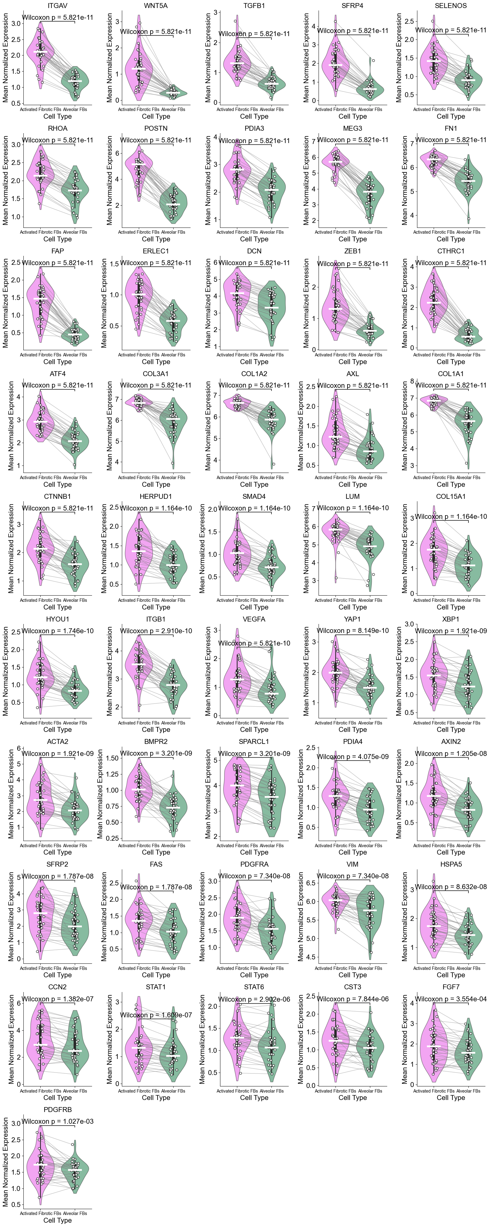
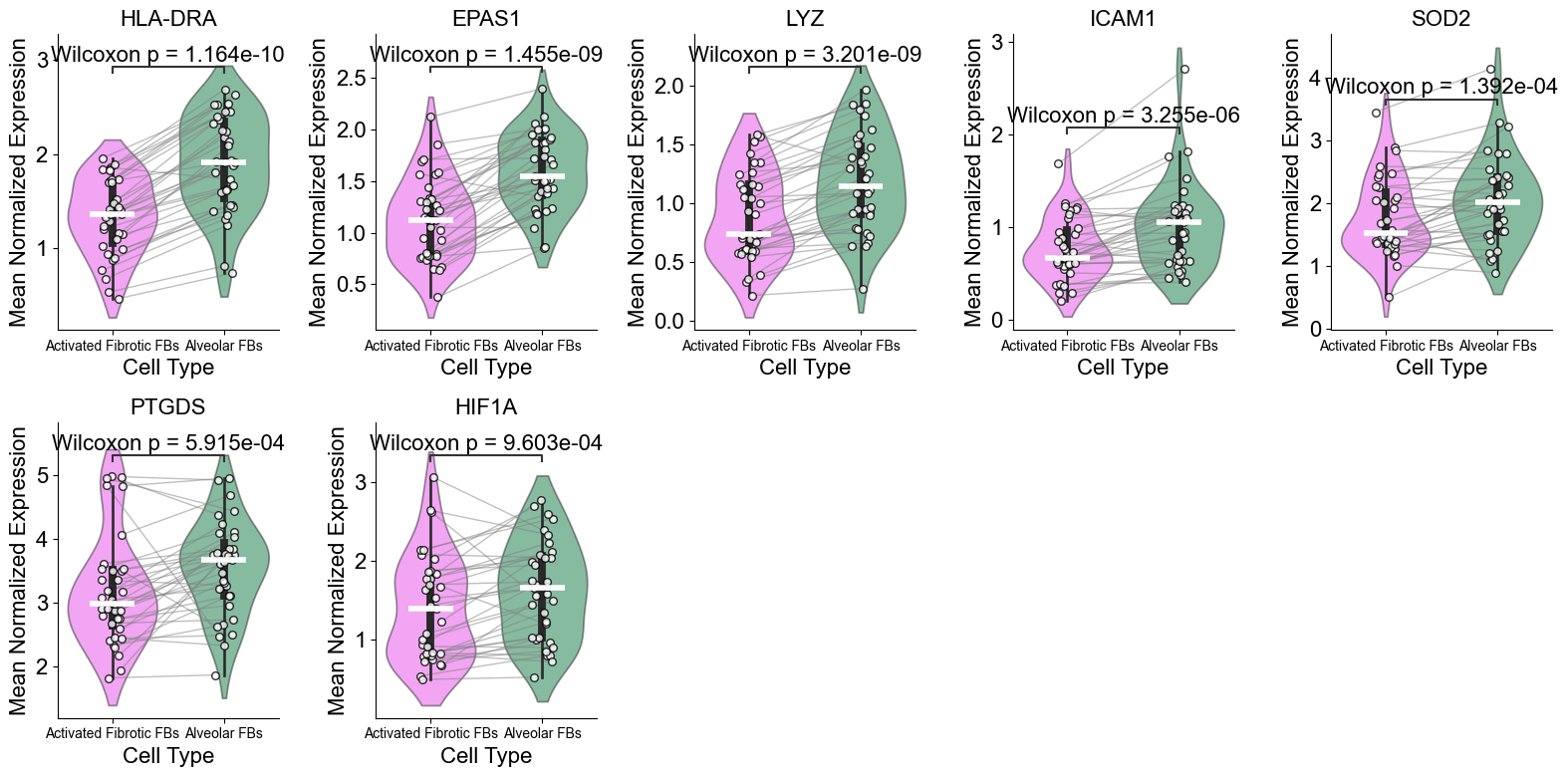
Compare activated fibrotic FBs and alveolar FBs within niche 5 (R1). For each slice, compute mean gene expression for each cell type, perform paired Wilcoxon tests, determine which cell type shows higher expression, and identify significant DEGs after FDR correction.
[43]:
from scipy.stats import wilcoxon, mannwhitneyu
from statsmodels.stats.multitest import multipletests
from scipy.stats import rankdata
from statannotations.Annotator import Annotator
np.random.seed(1234)

noi = '5'
ctoi_list = ['Activated Fibrotic FBs', 'Alveolar FBs']
min_cells = 20

qval_thres = 0.01
med_thres = 1

genes_list = cond_concat_new.var_names.tolist()
n_genes = len(genes_list)

avg_expr_noi1 = [[] for _ in range(n_genes)]
avg_expr_noi2 = [[] for _ in range(n_genes)]

for i, slice_name in enumerate(cond_name_list):

    adata = cond_concat_new[cond_concat_new.obs['slice_name'] == slice_name, :].copy()
    sc.pp.normalize_total(adata, target_sum=1e4)
    sc.pp.log1p(adata)

    adata_noi1 = adata[(adata.obs['final_CT'] == ctoi_list[0]) & (adata.obs['niche_label'] == noi), :].copy()
    adata_noi2 = adata[(adata.obs['final_CT'] == ctoi_list[1]) & (adata.obs['niche_label'] == noi), :].copy()

    n_cell_noi1 = adata_noi1.shape[0]
    n_cell_noi2 = adata_noi2.shape[0]

    if min(n_cell_noi1, n_cell_noi2) < min_cells:
        print(f"Skip {slice_name} due to rare cell count ({n_cell_noi1} vs {n_cell_noi2}).")
        continue

    for j, gene in enumerate(genes_list):
        avg_expr_noi1[j].append(np.mean(adata_noi1[:, gene].X))
        avg_expr_noi2[j].append(np.mean(adata_noi2[:, gene].X))

results = []
for j, gene in enumerate(genes_list):
    vals1 = np.array(avg_expr_noi1[j])
    vals2 = np.array(avg_expr_noi2[j])

    stat, pval = wilcoxon(vals1, vals2)

    diff = vals1 - vals2
    non_zero_mask = diff != 0
    diff_non_zero = diff[non_zero_mask]
    abs_diff = np.abs(diff_non_zero)
    ranks = rankdata(abs_diff)
    W_plus = np.sum(ranks[diff_non_zero > 0])
    W_minus = np.sum(ranks[diff_non_zero < 0])
    if W_plus > W_minus:
        greater=ctoi_list[0]
    else:
        greater=ctoi_list[1]

    results.append({
        'gene': gene,
        'stat': stat,
        'p-value': pval,
        'greater': greater,
        'median1': np.median(vals1),
        'median2': np.median(vals2),
        'median_max': max(np.median(vals1), np.median(vals2))
    })

df_results = pd.DataFrame(results)

df_results['q-value'] = multipletests(df_results['p-value'], method='fdr_bh')[1]

df_results['deg'] = 'FALSE'
# df_results.loc[(df_results['q-value'] < qval_thres) & (df_results['greater'] == ctoi_list[0]), 'deg'] = ctoi_list[0]
# df_results.loc[(df_results['q-value'] < qval_thres) & (df_results['greater'] == ctoi_list[1]), 'deg'] = ctoi_list[1]
df_results.loc[(df_results['q-value'] < qval_thres), 'deg'] = df_results.loc[(df_results['q-value'] < qval_thres) &
                                                                             (df_results['median_max'] > med_thres), 'greater']

df_deg_1 = df_results[df_results['deg'] == ctoi_list[0]].copy()
df_deg_1 = df_deg_1.sort_values('q-value', ascending=True)
df_deg_2 = df_results[df_results['deg'] == ctoi_list[1]].copy()
df_deg_2 = df_deg_2.sort_values('q-value', ascending=True)
CTHRC1, WNT5A, TGFB1, SFRP2, SFRP4, POSTN, SMAD4, FN1, CTNNB1, PDIA3, BMPR2, CCN2, ACTA2, PDGFRA, AXIN2, FGF7, COL1A1, COL1A2, COL3A1, COL15A1
[44]:
np.random.seed(1234)

gene_list = df_deg_1['gene'].tolist()
print(gene_list)
n_genes = len(gene_list)

ncol = 5
nrow = int(np.ceil(n_genes / ncol))
fig, axes = plt.subplots(nrow, ncol, figsize=(3.2*ncol, 4*nrow))
axes = axes.flatten()

for j, gene in enumerate(gene_list):

    g_idx = df_results.index[df_results['gene'] == gene][0]

    vals1 = avg_expr_noi1[g_idx]
    vals2 = avg_expr_noi2[g_idx]
    ax = axes[j]

    df_plot = pd.DataFrame({
        'expr': np.concatenate([vals1, vals2]),
        'group': [ctoi_list[0]]*len(vals1)
               + [ctoi_list[1]]*len(vals2)
    })

    colors = [ct_color_dict[ctoi_list[0]], ct_color_dict[ctoi_list[1]]]
    sns.violinplot(x='group', y='expr', data=df_plot, ax=ax, palette=colors, cut=1, inner='box', width=0.8, alpha=0.5)

    for xpos, vals in zip([0,1],[vals1, vals2]):
        ax.hlines(np.median(vals), xpos-0.2, xpos+0.2,
                  color='white', lw=4, zorder=3)

    pairs = [(ctoi_list[0], ctoi_list[1])]
    annot = Annotator(ax, pairs, data=df_plot, x='group', y='expr')
    annot.configure(test='Wilcoxon', text_format='full', loc='inside', verbose=0, fontsize=16,)
    annot.apply_and_annotate()

    ax.set_title(gene, fontsize=14)
    ax.set_ylabel('mean normalized expression', fontsize=12)
    ax.set_xlabel('')
    ax.grid(False)
    for k in range(len(vals1)):
        jitter = 0.1
        xx1 = 0 + np.random.uniform(-jitter, jitter)
        xx2 = 1 + np.random.uniform(-jitter, jitter)
        ax.plot([xx1, xx2], [vals1[k], vals2[k]], color='gray', linewidth=1, alpha=0.5, zorder=1)
        ax.scatter(xx1, vals1[k], color='white', s=30, alpha=0.8, edgecolor='black', zorder=2)
        ax.scatter(xx2, vals2[k], color='white', s=30, alpha=0.8, edgecolor='black', zorder=2)

    ax.set_xticklabels([ctoi_list[0], ctoi_list[1]], fontsize=10)
    ax.tick_params(axis='y', labelsize=16)
    ax.set_title(gene, fontsize=16)
    ax.set_ylabel('Mean Normalized Expression', fontsize=16)
    ax.set_xlabel('Cell Type', fontsize=16)
    ax.grid(False)
    ax.spines['top'].set_visible(False)
    ax.spines['right'].set_visible(False)

for ax in axes[j+1:]:
    ax.axis('off')

print(f"({ctoi_list[0]} vs {ctoi_list[1]}) (niche {noi})")
plt.tight_layout()
plt.show()
['ITGAV', 'WNT5A', 'TGFB1', 'SFRP4', 'SELENOS', 'RHOA', 'POSTN', 'PDIA3', 'MEG3', 'FN1', 'FAP', 'ERLEC1', 'DCN', 'ZEB1', 'CTHRC1', 'ATF4', 'COL3A1', 'COL1A2', 'AXL', 'COL1A1', 'CTNNB1', 'HERPUD1', 'SMAD4', 'LUM', 'COL15A1', 'HYOU1', 'ITGB1', 'VEGFA', 'YAP1', 'XBP1', 'ACTA2', 'BMPR2', 'SPARCL1', 'PDIA4', 'AXIN2', 'SFRP2', 'FAS', 'PDGFRA', 'VIM', 'HSPA5', 'CCN2', 'STAT1', 'STAT6', 'CST3', 'FGF7', 'PDGFRB']
(Activated Fibrotic FBs vs Alveolar FBs) (niche 5)
[45]:
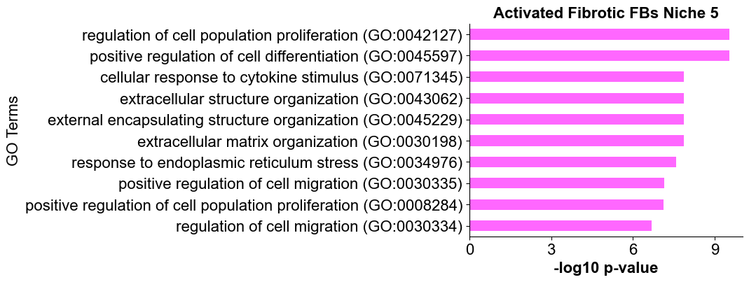
gene_list = df_deg_1['gene'].tolist()

enr = gp.enrichr(gene_list=gene_list,
                gene_sets=['GO_Biological_Process_2021'],
                organism='Human',
                outdir=None,
                # outdir=save_dir+f'{ctoi_list[0]}_niche{noi}_go_results',
                cutoff=0.05,
                )

ax = gp.barplot(
    enr.results,
    title=ctoi_list[0],
    cutoff=0.05,
    color=colors[0],
    figsize=(5, 4),
)

ax.set_title(f'{ctoi_list[0]} Niche {noi}', fontsize=16, fontweight='bold')
ax.set_xlabel('-log10 p-value', fontsize=16)
ax.set_ylabel('GO Terms', fontsize=16)
ax.grid(False)

plt.tight_layout()
plt.show()
[46]:
np.random.seed(1234)
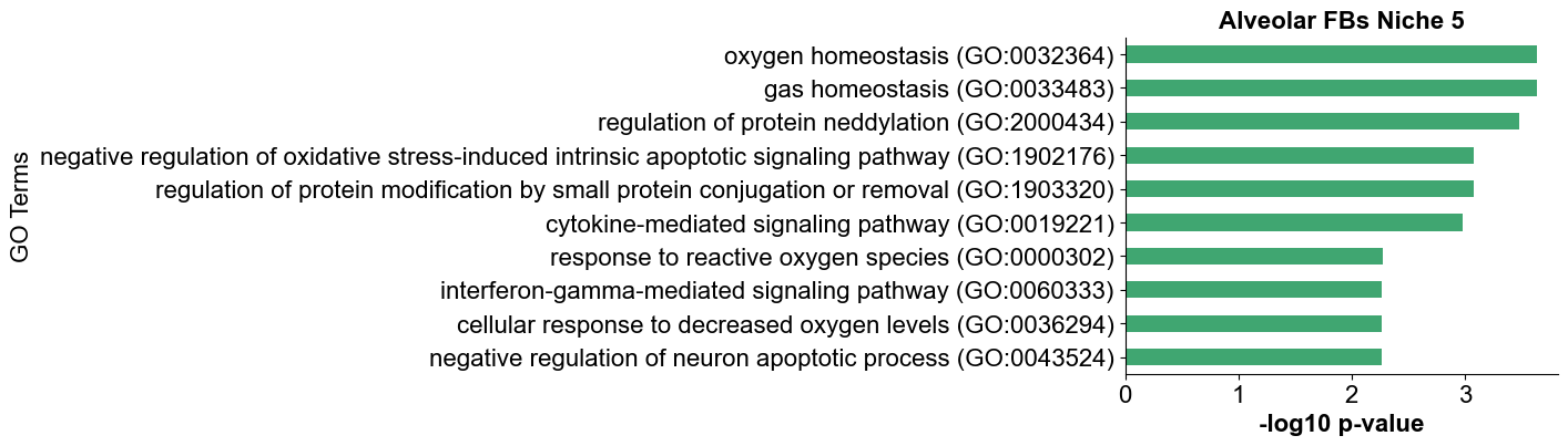
gene_list = df_deg_2['gene'].tolist()
print(gene_list)
n_genes = len(gene_list)
ncol = 5
nrow = int(np.ceil(n_genes / ncol))
fig, axes = plt.subplots(nrow, ncol, figsize=(3.2*ncol, 4*nrow))
axes = axes.flatten()
for j, gene in enumerate(gene_list):
g_idx = df_results.index[df_results['gene'] == gene][0]
vals1 = avg_expr_noi1[g_idx]
vals2 = avg_expr_noi2[g_idx]
ax = axes[j]
df_plot = pd.DataFrame({
'expr': np.concatenate([vals1, vals2]),
'group': [ctoi_list[0]]*len(vals1)
+ [ctoi_list[1]]*len(vals2)
})
colors = [ct_color_dict[ctoi_list[0]], ct_color_dict[ctoi_list[1]]]
sns.violinplot(x='group', y='expr', data=df_plot, ax=ax, palette=colors, cut=1, inner='box', width=0.8, alpha=0.5)
for xpos, vals in zip([0,1],[vals1, vals2]):
ax.hlines(np.median(vals), xpos-0.2, xpos+0.2,
color='white', lw=4, zorder=3)
pairs = [(ctoi_list[0], ctoi_list[1])]
annot = Annotator(ax, pairs, data=df_plot, x='group', y='expr')
annot.configure(test='Wilcoxon', text_format='full', loc='inside', verbose=0, fontsize=16,)
annot.apply_and_annotate()
ax.set_title(gene, fontsize=14)
ax.set_ylabel('mean normalized expression', fontsize=12)
ax.set_xlabel('')
ax.grid(False)
for k in range(len(vals1)):
jitter = 0.1
xx1 = 0 + np.random.uniform(-jitter, jitter)
xx2 = 1 + np.random.uniform(-jitter, jitter)
ax.plot([xx1, xx2], [vals1[k], vals2[k]], color='gray', linewidth=1, alpha=0.5, zorder=1)
ax.scatter(xx1, vals1[k], color='white', s=30, alpha=0.8, edgecolor='black', zorder=2)
ax.scatter(xx2, vals2[k], color='white', s=30, alpha=0.8, edgecolor='black', zorder=2)
ax.set_xticklabels([ctoi_list[0], ctoi_list[1]], fontsize=10)
ax.tick_params(axis='y', labelsize=16)
ax.set_title(gene, fontsize=16)
ax.set_ylabel('Mean Normalized Expression', fontsize=16)
ax.set_xlabel('Cell Type', fontsize=16)
ax.spines['top'].set_visible(False)
ax.spines['right'].set_visible(False)
ax.grid(False)
for ax in axes[j+1:]:
ax.axis('off')
print(f"({ctoi_list[0]} vs {ctoi_list[1]}) (niche {noi})")
plt.tight_layout()
plt.show()
['HLA-DRA', 'EPAS1', 'LYZ', 'ICAM1', 'SOD2', 'PTGDS', 'HIF1A']
(Activated Fibrotic FBs vs Alveolar FBs) (niche 5)
[47]:
gene_list = df_deg_2['gene'].tolist()

enr = gp.enrichr(gene_list=gene_list,
                gene_sets=['GO_Biological_Process_2021'],
                organism='Human',
                outdir=None,
                # outdir=save_dir+f'{ctoi_list[1]}_niche{noi}_go_results',
                cutoff=0.05,
                )

ax = gp.barplot(
    enr.results,
    title=ctoi_list[1],
    cutoff=0.05,
    color=colors[1],
    figsize=(5, 4),
)

ax.set_title(f'{ctoi_list[1]} Niche {noi}', fontsize=16, fontweight='bold')
ax.set_xlabel('-log10 p-value', fontsize=16)
ax.set_ylabel('GO Terms', fontsize=16)
ax.grid(False)

plt.tight_layout()
plt.show()
Niche 6 (R2)
Basal cells
Compare Basal cells across two niches (6 and 1). For each slice, compute mean gene expression within each niche, perform paired Wilcoxon tests to determine which niche shows higher expression, and identify significant DEGs after FDR correction.
[13]:
from scipy.stats import wilcoxon, mannwhitneyu
from statsmodels.stats.multitest import multipletests
from scipy.stats import rankdata
from statannotations.Annotator import Annotator
np.random.seed(1234)

noi_list = ['6', '1']
ctoi = 'Basal'
min_cells = 20

qval_thres = 0.01
med_thres = 0

genes_list = cond_concat_new.var_names.tolist()
n_genes = len(genes_list)

avg_expr_noi1 = [[] for _ in range(n_genes)]
avg_expr_noi2 = [[] for _ in range(n_genes)]

for i, slice_name in enumerate(cond_name_list):

    adata = cond_concat_new[cond_concat_new.obs['slice_name'] == slice_name, :].copy()
    sc.pp.normalize_total(adata, target_sum=1e4)
    sc.pp.log1p(adata)

    adata_noi1 = adata[(adata.obs['final_CT'] == ctoi) & (adata.obs['niche_label'] == noi_list[0]), :].copy()
    adata_noi2 = adata[(adata.obs['final_CT'] == ctoi) & (adata.obs['niche_label'] == noi_list[1]), :].copy()

    n_cell_noi1 = adata_noi1.shape[0]
    n_cell_noi2 = adata_noi2.shape[0]

    if min(n_cell_noi1, n_cell_noi2) < min_cells:
        print(f"Skip {slice_name} due to rare cell count ({n_cell_noi1} vs {n_cell_noi2}).")
        continue

    for j, gene in enumerate(genes_list):
        avg_expr_noi1[j].append(np.mean(adata_noi1[:, gene].X))
        avg_expr_noi2[j].append(np.mean(adata_noi2[:, gene].X))

results = []
for j, gene in enumerate(genes_list):
    vals1 = np.array(avg_expr_noi1[j])
    vals2 = np.array(avg_expr_noi2[j])

    stat, pval = wilcoxon(vals1, vals2)

    diff = vals1 - vals2
    non_zero_mask = diff != 0
    diff_non_zero = diff[non_zero_mask]
    abs_diff = np.abs(diff_non_zero)
    ranks = rankdata(abs_diff)
    W_plus = np.sum(ranks[diff_non_zero > 0])
    W_minus = np.sum(ranks[diff_non_zero < 0])
    if W_plus > W_minus:
        greater=noi_list[0]
    else:
        greater=noi_list[1]

    results.append({
        'gene': gene,
        'stat': stat,
        'p-value': pval,
        'greater': greater,
        'median1': np.median(vals1),
        'median2': np.median(vals2),
        'median_max': max(np.median(vals1), np.median(vals2))
    })

df_results = pd.DataFrame(results)

df_results['q-value'] = multipletests(df_results['p-value'], method='fdr_bh')[1]

df_results['deg'] = 'FALSE'
# df_results.loc[(df_results['q-value'] < qval_thres) & (df_results['greater'] == noi_list[0]), 'deg'] = noi_list[0]
# df_results.loc[(df_results['q-value'] < qval_thres) & (df_results['greater'] == noi_list[1]), 'deg'] = noi_list[1]
df_results.loc[(df_results['q-value'] < qval_thres), 'deg'] = df_results.loc[(df_results['q-value'] < qval_thres) &
                                                                             (df_results['median_max'] > med_thres), 'greater']

df_deg_1 = df_results[df_results['deg'] == noi_list[0]].copy()
df_deg_1 = df_deg_1.sort_values('q-value', ascending=True)
df_deg_2 = df_results[df_results['deg'] == noi_list[1]].copy()
df_deg_2 = df_deg_2.sort_values('q-value', ascending=True)
Skip TILD028LA due to rare cell count (185 vs 7).
Skip TILD111LA due to rare cell count (0 vs 0).
Skip VUILD102LA due to rare cell count (0 vs 0).
Skip VUILD102MA due to rare cell count (0 vs 0).
Skip VUILD104MA1 due to rare cell count (42 vs 4).
Skip VUILD105MA1 due to rare cell count (12 vs 214).
Skip VUILD115MA due to rare cell count (20 vs 3).
Skip VUILD142MA due to rare cell count (104 vs 0).
Skip VUILD48LA1 due to rare cell count (0 vs 0).
Skip VUILD48LA2 due to rare cell count (32 vs 0).
Skip VUILD49LA due to rare cell count (1 vs 0).
Skip VUILD78LA due to rare cell count (496 vs 9).
Skip VUILD91MA due to rare cell count (2 vs 0).
KRT8, KRT5, KRT14, KRT6A, SFTPC, SFTPD, NAPSA, SFTA2, MMP7, FN1, ITGAV, ITGB6, CEACAM5, CEACAM6, RNASE1, CD44, VIM
[14]:
np.random.seed(1234)

gene_list = df_deg_1['gene'].tolist()
print(gene_list)
n_genes = len(gene_list)

ncol = 5
nrow = int(np.ceil(n_genes / ncol))
fig, axes = plt.subplots(nrow, ncol, figsize=(3.2*ncol, 4*nrow))
axes = axes.flatten()

for j, gene in enumerate(gene_list):

    g_idx = df_results.index[df_results['gene'] == gene][0]

    vals1 = avg_expr_noi1[g_idx]
    vals2 = avg_expr_noi2[g_idx]
    ax = axes[j]

    df_plot = pd.DataFrame({
        'expr': np.concatenate([vals1, vals2]),
        'group': [noi_list[0]]*len(vals1)
               + [noi_list[1]]*len(vals2)
    })

    colors = [ct_color_dict[ctoi], niche_color_dict[noi_list[1]]]
    sns.violinplot(x='group', y='expr', data=df_plot, ax=ax, palette=colors, cut=1, inner='box', width=0.8, alpha=0.5)

    for xpos, vals in zip([0,1],[vals1, vals2]):
        ax.hlines(np.median(vals), xpos-0.2, xpos+0.2,
                  color='white', lw=4, zorder=3)

    pairs = [(noi_list[0], noi_list[1])]
    annot = Annotator(ax, pairs, data=df_plot, x='group', y='expr')
    annot.configure(test='Wilcoxon', text_format='full', loc='inside', verbose=0, fontsize=16,)
    annot.apply_and_annotate()

    ax.set_title(gene, fontsize=14)
    ax.set_ylabel('mean normalized expression', fontsize=12)
    ax.set_xlabel('')
    ax.grid(False)
    for k in range(len(vals1)):
        jitter = 0.1
        xx1 = 0 + np.random.uniform(-jitter, jitter)
        xx2 = 1 + np.random.uniform(-jitter, jitter)
        ax.plot([xx1, xx2], [vals1[k], vals2[k]], color='gray', linewidth=1, alpha=0.5, zorder=1)
        ax.scatter(xx1, vals1[k], color='white', s=30, alpha=0.8, edgecolor='black', zorder=2)
        ax.scatter(xx2, vals2[k], color='white', s=30, alpha=0.8, edgecolor='black', zorder=2)

    ax.set_xticklabels([noi_list[0], noi_list[1]], fontsize=16)
    ax.tick_params(axis='y', labelsize=16)
    ax.set_title(gene, fontsize=16)
    ax.set_ylabel('Mean Normalized Expression', fontsize=16)
    ax.set_xlabel('Niche', fontsize=16)
    ax.spines['top'].set_visible(False)
    ax.spines['right'].set_visible(False)
    ax.grid(False)

for ax in axes[j+1:]:
    ax.axis('off')

print(f"{ctoi} (niche {noi_list[0]} vs niche {noi_list[1]})")
plt.tight_layout()
plt.show()
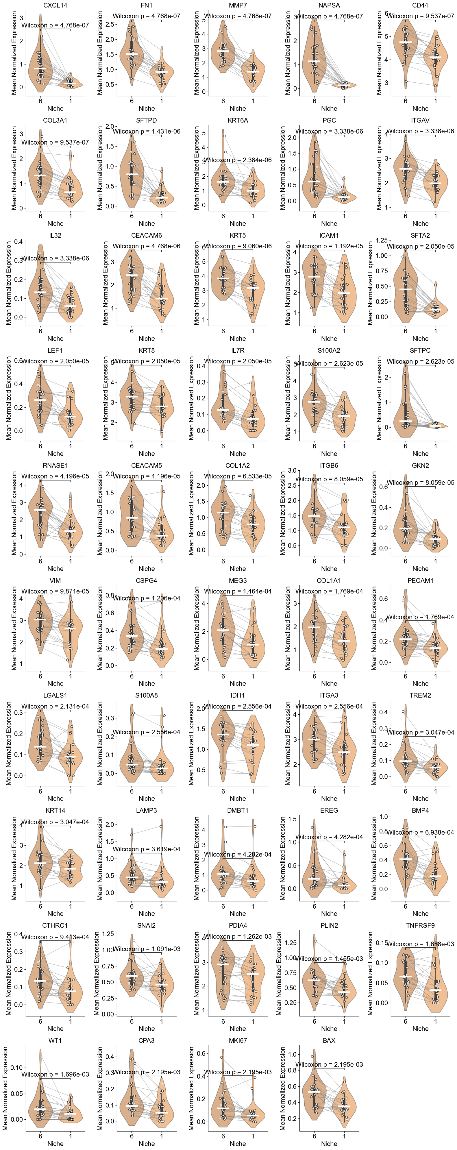
['CXCL14', 'FN1', 'MMP7', 'NAPSA', 'CD44', 'COL3A1', 'SFTPD', 'KRT6A', 'PGC', 'ITGAV', 'IL32', 'CEACAM6', 'KRT5', 'ICAM1', 'SFTA2', 'LEF1', 'KRT8', 'IL7R', 'S100A2', 'SFTPC', 'RNASE1', 'CEACAM5', 'COL1A2', 'ITGB6', 'GKN2', 'VIM', 'CSPG4', 'MEG3', 'COL1A1', 'PECAM1', 'LGALS1', 'S100A8', 'IDH1', 'ITGA3', 'TREM2', 'KRT14', 'LAMP3', 'DMBT1', 'EREG', 'BMP4', 'CTHRC1', 'SNAI2', 'PDIA4', 'PLIN2', 'TNFRSF9', 'WT1', 'CPA3', 'MKI67', 'BAX']
Basal (niche 6 vs niche 1)
TP63, SOX2, SCGB1A1
[15]:
np.random.seed(1234)

gene_list = df_deg_2['gene'].tolist()
print(gene_list)
n_genes = len(gene_list)

ncol = 5
nrow = int(np.ceil(n_genes / ncol))
fig, axes = plt.subplots(nrow, ncol, figsize=(3.2*ncol, 4*nrow))
axes = axes.flatten()

for j, gene in enumerate(gene_list):

    g_idx = df_results.index[df_results['gene'] == gene][0]

    vals1 = avg_expr_noi1[g_idx]
    vals2 = avg_expr_noi2[g_idx]
    ax = axes[j]

    df_plot = pd.DataFrame({
        'expr': np.concatenate([vals1, vals2]),
        'group': [noi_list[0]]*len(vals1)
               + [noi_list[1]]*len(vals2)
    })

    colors = [ct_color_dict[ctoi], niche_color_dict[noi_list[1]]]
    sns.violinplot(x='group', y='expr', data=df_plot, ax=ax, palette=colors, cut=1, inner='box', width=0.8, alpha=0.5)

    for xpos, vals in zip([0,1],[vals1, vals2]):
        ax.hlines(np.median(vals), xpos-0.2, xpos+0.2,
                  color='white', lw=4, zorder=3)

    pairs = [(noi_list[0], noi_list[1])]
    annot = Annotator(ax, pairs, data=df_plot, x='group', y='expr')
    annot.configure(test='Wilcoxon', text_format='full', loc='inside', verbose=0, fontsize=16,)
    annot.apply_and_annotate()

    ax.set_title(gene, fontsize=14)
    ax.set_ylabel('mean normalized expression', fontsize=12)
    ax.set_xlabel('')
    ax.grid(False)
    for k in range(len(vals1)):
        jitter = 0.1
        xx1 = 0 + np.random.uniform(-jitter, jitter)
        xx2 = 1 + np.random.uniform(-jitter, jitter)
        ax.plot([xx1, xx2], [vals1[k], vals2[k]], color='gray', linewidth=1, alpha=0.5, zorder=1)
        ax.scatter(xx1, vals1[k], color='white', s=30, alpha=0.8, edgecolor='black', zorder=2)
        ax.scatter(xx2, vals2[k], color='white', s=30, alpha=0.8, edgecolor='black', zorder=2)

    ax.set_xticklabels([noi_list[0], noi_list[1]], fontsize=16)
    ax.tick_params(axis='y', labelsize=16)
    ax.set_title(gene, fontsize=16)
    ax.set_ylabel('Mean Normalized Expression', fontsize=16)
    ax.set_xlabel('Niche', fontsize=16)
    ax.spines['top'].set_visible(False)
    ax.spines['right'].set_visible(False)
    ax.grid(False)

for ax in axes[j+1:]:
    ax.axis('off')

print(f"{ctoi} (niche {noi_list[0]} vs niche {noi_list[1]})")
plt.tight_layout()
plt.show()
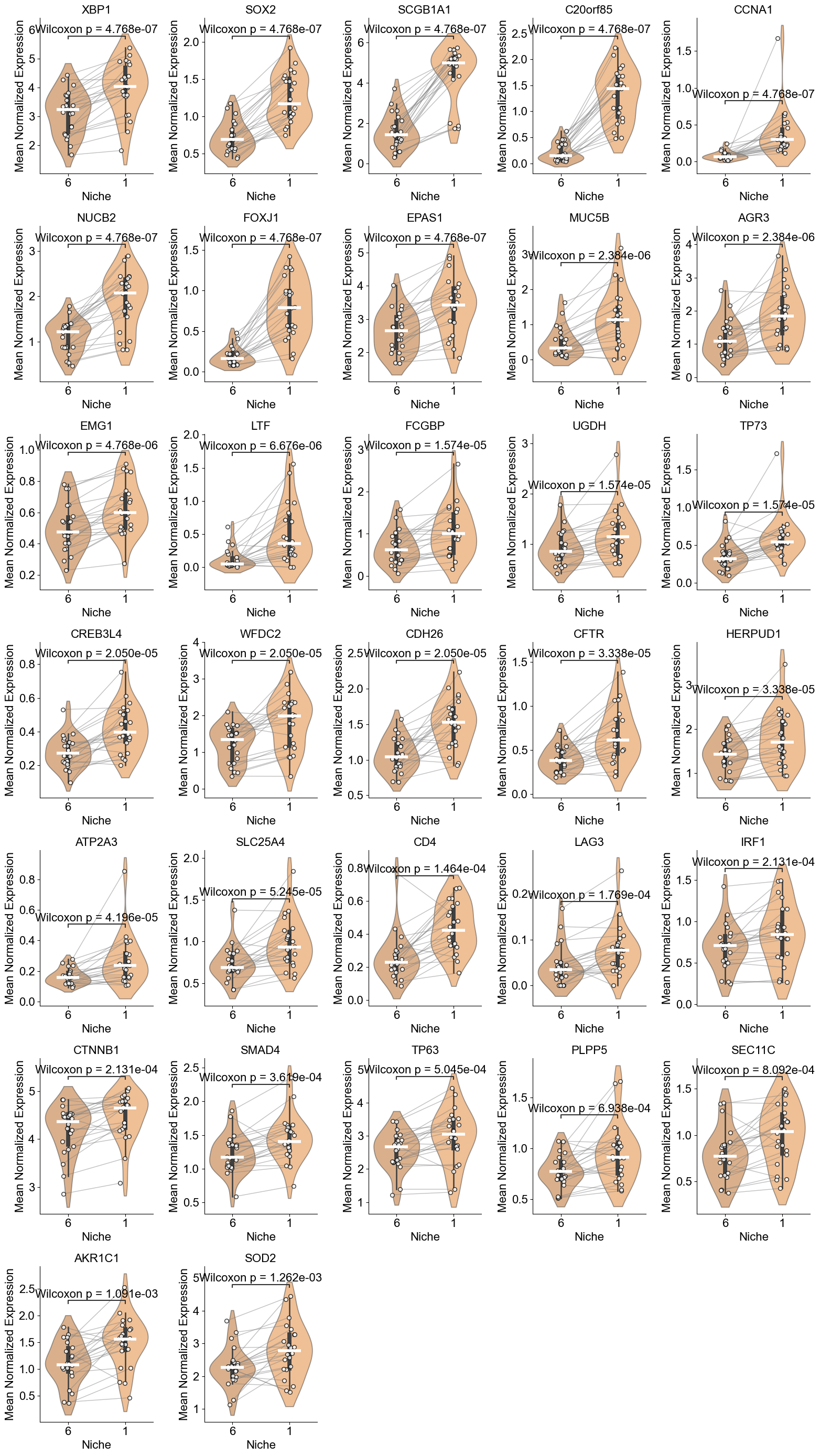
['XBP1', 'SOX2', 'SCGB1A1', 'C20orf85', 'CCNA1', 'NUCB2', 'FOXJ1', 'EPAS1', 'MUC5B', 'AGR3', 'EMG1', 'LTF', 'FCGBP', 'UGDH', 'TP73', 'CREB3L4', 'WFDC2', 'CDH26', 'CFTR', 'HERPUD1', 'ATP2A3', 'SLC25A4', 'CD4', 'LAG3', 'IRF1', 'CTNNB1', 'SMAD4', 'TP63', 'PLPP5', 'SEC11C', 'AKR1C1', 'SOD2']
Basal (niche 6 vs niche 1)
RASC
Compare RASC cells across two niches (6 and 1). For each slice, calculate the mean gene expression within each niche, perform paired Wilcoxon tests to determine which niche exhibits higher expression, and identify significant DEGs after FDR correction.
[16]:
from scipy.stats import wilcoxon, mannwhitneyu
from statsmodels.stats.multitest import multipletests
from scipy.stats import rankdata
from statannotations.Annotator import Annotator
np.random.seed(1234)

noi_list = ['6', '1']
ctoi = 'RASC'
min_cells = 20

qval_thres = 0.01
med_thres = 0

genes_list = cond_concat_new.var_names.tolist()
n_genes = len(genes_list)

avg_expr_noi1 = [[] for _ in range(n_genes)]
avg_expr_noi2 = [[] for _ in range(n_genes)]

for i, slice_name in enumerate(cond_name_list):

    adata = cond_concat_new[cond_concat_new.obs['slice_name'] == slice_name, :].copy()
    sc.pp.normalize_total(adata, target_sum=1e4)
    sc.pp.log1p(adata)

    adata_noi1 = adata[(adata.obs['final_CT'] == ctoi) & (adata.obs['niche_label'] == noi_list[0]), :].copy()
    adata_noi2 = adata[(adata.obs['final_CT'] == ctoi) & (adata.obs['niche_label'] == noi_list[1]), :].copy()

    n_cell_noi1 = adata_noi1.shape[0]
    n_cell_noi2 = adata_noi2.shape[0]

    if min(n_cell_noi1, n_cell_noi2) < min_cells:
        print(f"Skip {slice_name} due to rare cell count ({n_cell_noi1} vs {n_cell_noi2}).")
        continue

    for j, gene in enumerate(genes_list):
        avg_expr_noi1[j].append(np.mean(adata_noi1[:, gene].X))
        avg_expr_noi2[j].append(np.mean(adata_noi2[:, gene].X))

results = []
for j, gene in enumerate(genes_list):
    vals1 = np.array(avg_expr_noi1[j])
    vals2 = np.array(avg_expr_noi2[j])

    stat, pval = wilcoxon(vals1, vals2)

    diff = vals1 - vals2
    non_zero_mask = diff != 0
    diff_non_zero = diff[non_zero_mask]
    abs_diff = np.abs(diff_non_zero)
    ranks = rankdata(abs_diff)
    W_plus = np.sum(ranks[diff_non_zero > 0])
    W_minus = np.sum(ranks[diff_non_zero < 0])
    if W_plus > W_minus:
        greater=noi_list[0]
    else:
        greater=noi_list[1]

    results.append({
        'gene': gene,
        'stat': stat,
        'p-value': pval,
        'greater': greater,
        'median1': np.median(vals1),
        'median2': np.median(vals2),
        'median_max': max(np.median(vals1), np.median(vals2))
    })

df_results = pd.DataFrame(results)

df_results['q-value'] = multipletests(df_results['p-value'], method='fdr_bh')[1]

df_results['deg'] = 'FALSE'
# df_results.loc[(df_results['q-value'] < qval_thres) & (df_results['greater'] == noi_list[0]), 'deg'] = noi_list[0]
# df_results.loc[(df_results['q-value'] < qval_thres) & (df_results['greater'] == noi_list[1]), 'deg'] = noi_list[1]
df_results.loc[(df_results['q-value'] < qval_thres), 'deg'] = df_results.loc[(df_results['q-value'] < qval_thres) &
                                                                             (df_results['median_max'] > med_thres), 'greater']

df_deg_1 = df_results[df_results['deg'] == noi_list[0]].copy()
df_deg_1 = df_deg_1.sort_values('q-value', ascending=True)
df_deg_2 = df_results[df_results['deg'] == noi_list[1]].copy()
df_deg_2 = df_deg_2.sort_values('q-value', ascending=True)
Skip TILD028LA due to rare cell count (136 vs 2).
Skip TILD111LA due to rare cell count (1 vs 0).
Skip TILD130LA due to rare cell count (106 vs 12).
Skip TILD299MA due to rare cell count (62 vs 17).
Skip VUILD102LA due to rare cell count (0 vs 0).
Skip VUILD102MA due to rare cell count (0 vs 0).
Skip VUILD104MA1 due to rare cell count (36 vs 4).
Skip VUILD105MA1 due to rare cell count (2 vs 0).
Skip VUILD115MA due to rare cell count (326 vs 5).
Skip VUILD142MA due to rare cell count (13 vs 0).
Skip VUILD48LA1 due to rare cell count (0 vs 0).
Skip VUILD48LA2 due to rare cell count (5 vs 0).
Skip VUILD49LA due to rare cell count (0 vs 0).
Skip VUILD78LA due to rare cell count (345 vs 9).
Skip VUILD91LA due to rare cell count (112 vs 17).
Skip VUILD91MA due to rare cell count (5 vs 0).
SFTPD, CD44, NAPSA, FN1, NKX2-1, RNASE1, SFTPC, SFTA2, ITGB6
[17]:
np.random.seed(1234)

gene_list = df_deg_1['gene'].tolist()
print(gene_list)
n_genes = len(gene_list)

ncol = 5
nrow = int(np.ceil(n_genes / ncol))
fig, axes = plt.subplots(nrow, ncol, figsize=(3.2*ncol, 4*nrow))
axes = axes.flatten()

for j, gene in enumerate(gene_list):

    g_idx = df_results.index[df_results['gene'] == gene][0]

    vals1 = avg_expr_noi1[g_idx]
    vals2 = avg_expr_noi2[g_idx]
    ax = axes[j]

    df_plot = pd.DataFrame({
        'expr': np.concatenate([vals1, vals2]),
        'group': [noi_list[0]]*len(vals1)
               + [noi_list[1]]*len(vals2)
    })

    colors = [ct_color_dict[ctoi], niche_color_dict[noi_list[1]]]
    sns.violinplot(x='group', y='expr', data=df_plot, ax=ax, palette=colors, cut=1, inner='box', width=0.8, alpha=0.5)

    for xpos, vals in zip([0,1],[vals1, vals2]):
        ax.hlines(np.median(vals), xpos-0.2, xpos+0.2,
                  color='white', lw=4, zorder=3)

    pairs = [(noi_list[0], noi_list[1])]
    annot = Annotator(ax, pairs, data=df_plot, x='group', y='expr')
    annot.configure(test='Wilcoxon', text_format='full', loc='inside', verbose=0, fontsize=16,)
    annot.apply_and_annotate()

    ax.set_title(gene, fontsize=14)
    ax.set_ylabel('mean normalized expression', fontsize=12)
    ax.set_xlabel('')
    ax.grid(False)
    for k in range(len(vals1)):
        jitter = 0.1
        xx1 = 0 + np.random.uniform(-jitter, jitter)
        xx2 = 1 + np.random.uniform(-jitter, jitter)
        ax.plot([xx1, xx2], [vals1[k], vals2[k]], color='gray', linewidth=1, alpha=0.5, zorder=1)
        ax.scatter(xx1, vals1[k], color='white', s=30, alpha=0.8, edgecolor='black', zorder=2)
        ax.scatter(xx2, vals2[k], color='white', s=30, alpha=0.8, edgecolor='black', zorder=2)

    ax.set_xticklabels([noi_list[0], noi_list[1]], fontsize=16)
    ax.tick_params(axis='y', labelsize=16)
    ax.set_title(gene, fontsize=16)
    ax.set_ylabel('Mean Normalized Expression', fontsize=16)
    ax.set_xlabel('Niche', fontsize=16)
    ax.spines['top'].set_visible(False)
    ax.spines['right'].set_visible(False)
    ax.grid(False)

for ax in axes[j+1:]:
    ax.axis('off')

print(f"{ctoi} (niche {noi_list[0]} vs niche {noi_list[1]})")
plt.tight_layout()
plt.show()
['SFTPD', 'CD44', 'NAPSA', 'HLA-DQB1', 'MSLN', 'BMP4', 'COL3A1', 'FN1', 'COL1A2', 'PGC', 'NKX2-1', 'ICAM1', 'DUOX1', 'RNASE1', 'SFTPC', 'HLA-DQA1', 'SCGB3A2', 'SFTA2', 'ITGB6', 'AIF1', 'CXCL14', 'S100A2']
RASC (niche 6 vs niche 1)
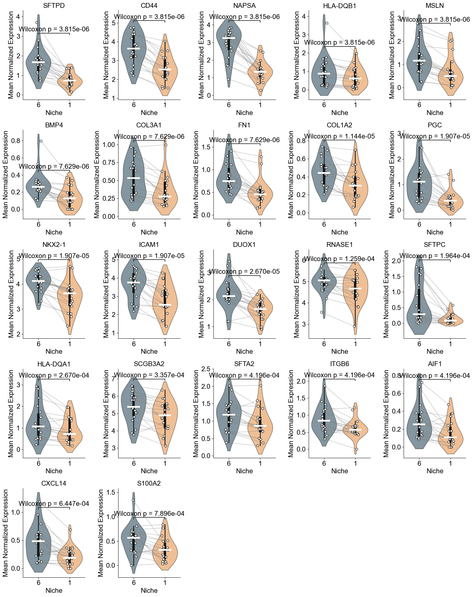
SCGB1A1, SOX2
[18]:
np.random.seed(1234)

gene_list = df_deg_2['gene'].tolist()
print(gene_list)
n_genes = len(gene_list)

ncol = 5
nrow = int(np.ceil(n_genes / ncol))
fig, axes = plt.subplots(nrow, ncol, figsize=(3.2*ncol, 4*nrow))
axes = axes.flatten()

for j, gene in enumerate(gene_list):

    g_idx = df_results.index[df_results['gene'] == gene][0]

    vals1 = avg_expr_noi1[g_idx]
    vals2 = avg_expr_noi2[g_idx]
    ax = axes[j]

    df_plot = pd.DataFrame({
        'expr': np.concatenate([vals1, vals2]),
        'group': [noi_list[0]]*len(vals1)
               + [noi_list[1]]*len(vals2)
    })

    colors = [ct_color_dict[ctoi], niche_color_dict[noi_list[1]]]
    sns.violinplot(x='group', y='expr', data=df_plot, ax=ax, palette=colors, cut=1, inner='box', width=0.8, alpha=0.5)

    for xpos, vals in zip([0,1],[vals1, vals2]):
        ax.hlines(np.median(vals), xpos-0.2, xpos+0.2,
                  color='white', lw=4, zorder=3)

    pairs = [(noi_list[0], noi_list[1])]
    annot = Annotator(ax, pairs, data=df_plot, x='group', y='expr')
    annot.configure(test='Wilcoxon', text_format='full', loc='inside', verbose=0, fontsize=16,)
    annot.apply_and_annotate()

    ax.set_title(gene, fontsize=14)
    ax.set_ylabel('mean normalized expression', fontsize=12)
    ax.set_xlabel('')
    ax.grid(False)
    for k in range(len(vals1)):
        jitter = 0.1
        xx1 = 0 + np.random.uniform(-jitter, jitter)
        xx2 = 1 + np.random.uniform(-jitter, jitter)
        ax.plot([xx1, xx2], [vals1[k], vals2[k]], color='gray', linewidth=1, alpha=0.5, zorder=1)
        ax.scatter(xx1, vals1[k], color='white', s=30, alpha=0.8, edgecolor='black', zorder=2)
        ax.scatter(xx2, vals2[k], color='white', s=30, alpha=0.8, edgecolor='black', zorder=2)

    ax.set_xticklabels([noi_list[0], noi_list[1]], fontsize=16)
    ax.tick_params(axis='y', labelsize=16)
    ax.set_title(gene, fontsize=16)
    ax.set_ylabel('Mean Normalized Expression', fontsize=16)
    ax.set_xlabel('Niche', fontsize=16)
    ax.spines['top'].set_visible(False)
    ax.spines['right'].set_visible(False)
    ax.grid(False)

for ax in axes[j+1:]:
    ax.axis('off')

print(f"{ctoi} (niche {noi_list[0]} vs niche {noi_list[1]})")
plt.tight_layout()
plt.show()
['FOXJ1', 'SCGB1A1', 'XBP1', 'C20orf85', 'SOX2', 'CCNA1', 'KDR', 'SOX4', 'NUCB2']
RASC (niche 6 vs niche 1)
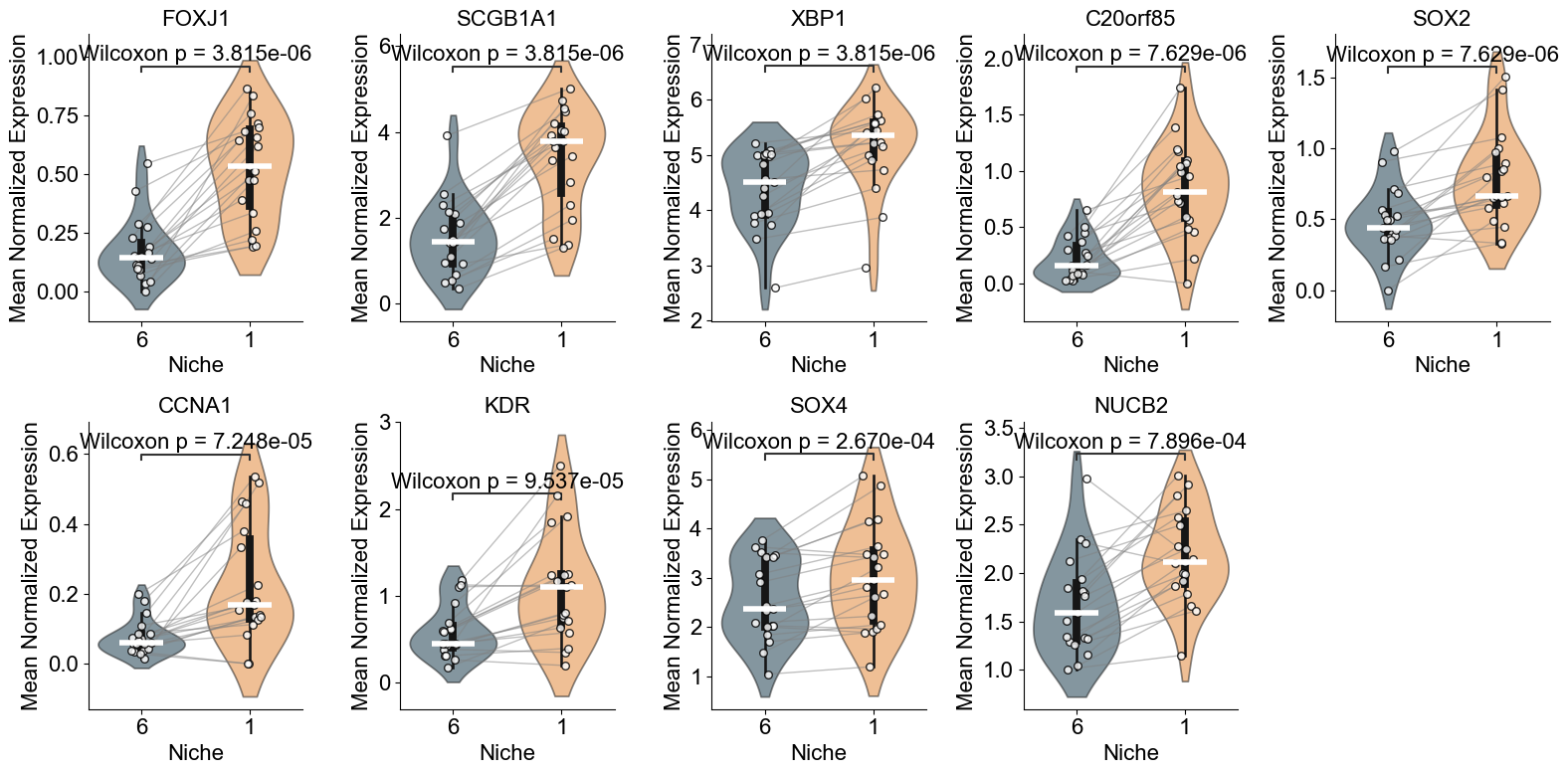
AT2
Compare AT2 cells between two niches (6 and 0). For each slice, mean gene expression is computed within each niche, paired Wilcoxon tests are performed to determine which niche has higher expression, and significant DEGs are identified after FDR correction.
[19]:
from scipy.stats import wilcoxon, mannwhitneyu
from statsmodels.stats.multitest import multipletests
from scipy.stats import rankdata
from statannotations.Annotator import Annotator
np.random.seed(1234)

noi_list = ['6', '0']
ctoi = 'AT2'
min_cells = 20

qval_thres = 0.01
med_thres = 0

genes_list = cond_concat_new.var_names.tolist()
n_genes = len(genes_list)

avg_expr_noi1 = [[] for _ in range(n_genes)]
avg_expr_noi2 = [[] for _ in range(n_genes)]

for i, slice_name in enumerate(cond_name_list):

    adata = cond_concat_new[cond_concat_new.obs['slice_name'] == slice_name, :].copy()
    sc.pp.normalize_total(adata, target_sum=1e4)
    sc.pp.log1p(adata)

    adata_noi1 = adata[(adata.obs['final_CT'] == ctoi) & (adata.obs['niche_label'] == noi_list[0]), :].copy()
    adata_noi2 = adata[(adata.obs['final_CT'] == ctoi) & (adata.obs['niche_label'] == noi_list[1]), :].copy()

    n_cell_noi1 = adata_noi1.shape[0]
    n_cell_noi2 = adata_noi2.shape[0]

    if min(n_cell_noi1, n_cell_noi2) < min_cells:
        print(f"Skip {slice_name} due to rare cell count ({n_cell_noi1} vs {n_cell_noi2}).")
        continue

    for j, gene in enumerate(genes_list):
        avg_expr_noi1[j].append(np.mean(adata_noi1[:, gene].X))
        avg_expr_noi2[j].append(np.mean(adata_noi2[:, gene].X))

results = []
for j, gene in enumerate(genes_list):
    vals1 = np.array(avg_expr_noi1[j])
    vals2 = np.array(avg_expr_noi2[j])

    stat, pval = wilcoxon(vals1, vals2)

    diff = vals1 - vals2
    non_zero_mask = diff != 0
    diff_non_zero = diff[non_zero_mask]
    abs_diff = np.abs(diff_non_zero)
    ranks = rankdata(abs_diff)
    W_plus = np.sum(ranks[diff_non_zero > 0])
    W_minus = np.sum(ranks[diff_non_zero < 0])
    if W_plus > W_minus:
        greater=noi_list[0]
    else:
        greater=noi_list[1]

    results.append({
        'gene': gene,
        'stat': stat,
        'p-value': pval,
        'greater': greater,
        'median1': np.median(vals1),
        'median2': np.median(vals2),
        'median_max': max(np.median(vals1), np.median(vals2))
    })

df_results = pd.DataFrame(results)

df_results['q-value'] = multipletests(df_results['p-value'], method='fdr_bh')[1]

df_results['deg'] = 'FALSE'
# df_results.loc[(df_results['q-value'] < qval_thres) & (df_results['greater'] == noi_list[0]), 'deg'] = noi_list[0]
# df_results.loc[(df_results['q-value'] < qval_thres) & (df_results['greater'] == noi_list[1]), 'deg'] = noi_list[1]
df_results.loc[(df_results['q-value'] < qval_thres), 'deg'] = df_results.loc[(df_results['q-value'] < qval_thres) &
                                                                             (df_results['median_max'] > med_thres), 'greater']

df_deg_1 = df_results[df_results['deg'] == noi_list[0]].copy()
df_deg_1 = df_deg_1.sort_values('q-value', ascending=True)
df_deg_2 = df_results[df_results['deg'] == noi_list[1]].copy()
df_deg_2 = df_deg_2.sort_values('q-value', ascending=True)
Skip TILD049MA due to rare cell count (30 vs 1).
Skip TILD111LA due to rare cell count (3 vs 1066).
Skip TILD117MA2 due to rare cell count (626 vs 16).
Skip TILD175MA due to rare cell count (182 vs 15).
Skip VUILD102LA due to rare cell count (0 vs 2702).
Skip VUILD102MA due to rare cell count (0 vs 1641).
Skip VUILD105MA1 due to rare cell count (7 vs 140).
Skip VUILD105MA2 due to rare cell count (156 vs 0).
Skip VUILD48LA1 due to rare cell count (4 vs 987).
Skip VUILD49LA due to rare cell count (2 vs 638).
Skip VUILD91MA due to rare cell count (11 vs 432).
Skip VUILD96LA due to rare cell count (18 vs 2890).
Skip VUILD96MA due to rare cell count (7 vs 0).
CEACAM6, KRT17, MMP7, KRT15, SCGB3A2, SCGB1A1, CEACAM5, SOX4, WFDC2
[20]:
np.random.seed(1234)

gene_list = df_deg_1['gene'].tolist()
print(gene_list)
n_genes = len(gene_list)

ncol = 5
nrow = int(np.ceil(n_genes / ncol))
fig, axes = plt.subplots(nrow, ncol, figsize=(3.2*ncol, 4*nrow))
axes = axes.flatten()

for j, gene in enumerate(gene_list):

    g_idx = df_results.index[df_results['gene'] == gene][0]

    vals1 = avg_expr_noi1[g_idx]
    vals2 = avg_expr_noi2[g_idx]
    ax = axes[j]

    df_plot = pd.DataFrame({
        'expr': np.concatenate([vals1, vals2]),
        'group': [noi_list[0]]*len(vals1)
               + [noi_list[1]]*len(vals2)
    })

    colors = [ct_color_dict[ctoi], niche_color_dict[noi_list[1]]]
    sns.violinplot(x='group', y='expr', data=df_plot, ax=ax, palette=colors, cut=1, inner='box', width=0.8, alpha=0.5)

    for xpos, vals in zip([0,1],[vals1, vals2]):
        ax.hlines(np.median(vals), xpos-0.2, xpos+0.2,
                  color='white', lw=4, zorder=3)

    pairs = [(noi_list[0], noi_list[1])]
    annot = Annotator(ax, pairs, data=df_plot, x='group', y='expr')
    annot.configure(test='Wilcoxon', text_format='full', loc='inside', verbose=0, fontsize=16,)
    annot.apply_and_annotate()

    ax.set_title(gene, fontsize=14)
    ax.set_ylabel('mean normalized expression', fontsize=12)
    ax.set_xlabel('')
    ax.grid(False)
    for k in range(len(vals1)):
        jitter = 0.1
        xx1 = 0 + np.random.uniform(-jitter, jitter)
        xx2 = 1 + np.random.uniform(-jitter, jitter)
        ax.plot([xx1, xx2], [vals1[k], vals2[k]], color='gray', linewidth=1, alpha=0.5, zorder=1)
        ax.scatter(xx1, vals1[k], color='white', s=30, alpha=0.8, edgecolor='black', zorder=2)
        ax.scatter(xx2, vals2[k], color='white', s=30, alpha=0.8, edgecolor='black', zorder=2)

    ax.set_xticklabels([noi_list[0], noi_list[1]], fontsize=16)
    ax.tick_params(axis='y', labelsize=16)
    ax.set_title(gene, fontsize=16)
    ax.set_ylabel('Mean Normalized Expression', fontsize=16)
    ax.set_xlabel('Niche', fontsize=16)
    ax.spines['top'].set_visible(False)
    ax.spines['right'].set_visible(False)
    ax.grid(False)

for ax in axes[j+1:]:
    ax.axis('off')

print(f"{ctoi} (niche {noi_list[0]} vs niche {noi_list[1]})")
plt.tight_layout()
plt.show()
['CEACAM6', 'KRT17', 'MMP7', 'KRT15', 'SCGB3A2', 'SCGB1A1', 'CEACAM5', 'SOX4', 'WFDC2', 'ITM2C']
AT2 (niche 6 vs niche 0)
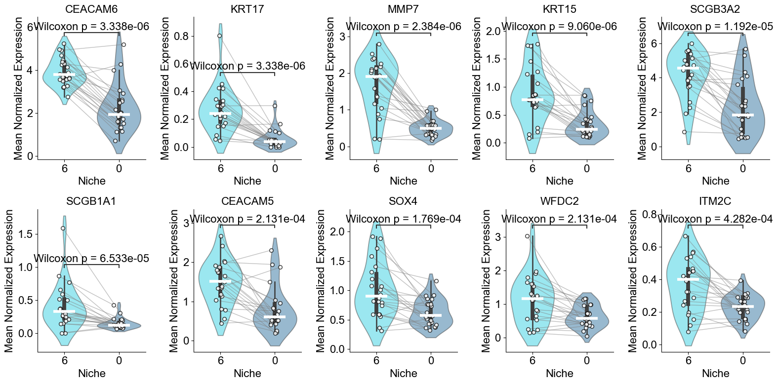
SFTPC, SFTPD, NAPSA, LAMP3
[21]:
np.random.seed(1234)

gene_list = df_deg_2['gene'].tolist()
print(gene_list)
n_genes = len(gene_list)

ncol = 5
nrow = int(np.ceil(n_genes / ncol))
fig, axes = plt.subplots(nrow, ncol, figsize=(3.2*ncol, 4*nrow))
axes = axes.flatten()

for j, gene in enumerate(gene_list):

    g_idx = df_results.index[df_results['gene'] == gene][0]

    vals1 = avg_expr_noi1[g_idx]
    vals2 = avg_expr_noi2[g_idx]
    ax = axes[j]

    df_plot = pd.DataFrame({
        'expr': np.concatenate([vals1, vals2]),
        'group': [noi_list[0]]*len(vals1)
               + [noi_list[1]]*len(vals2)
    })

    colors = [ct_color_dict[ctoi], niche_color_dict[noi_list[1]]]
    sns.violinplot(x='group', y='expr', data=df_plot, ax=ax, palette=colors, cut=1, inner='box', width=0.8, alpha=0.5)

    for xpos, vals in zip([0,1],[vals1, vals2]):
        ax.hlines(np.median(vals), xpos-0.2, xpos+0.2,
                  color='white', lw=4, zorder=3)

    pairs = [(noi_list[0], noi_list[1])]
    annot = Annotator(ax, pairs, data=df_plot, x='group', y='expr')
    annot.configure(test='Wilcoxon', text_format='full', loc='inside', verbose=0, fontsize=16,)
    annot.apply_and_annotate()

    ax.set_title(gene, fontsize=14)
    ax.set_ylabel('mean normalized expression', fontsize=12)
    ax.set_xlabel('')
    ax.grid(False)
    for k in range(len(vals1)):
        jitter = 0.1
        xx1 = 0 + np.random.uniform(-jitter, jitter)
        xx2 = 1 + np.random.uniform(-jitter, jitter)
        ax.plot([xx1, xx2], [vals1[k], vals2[k]], color='gray', linewidth=1, alpha=0.5, zorder=1)
        ax.scatter(xx1, vals1[k], color='white', s=30, alpha=0.8, edgecolor='black', zorder=2)
        ax.scatter(xx2, vals2[k], color='white', s=30, alpha=0.8, edgecolor='black', zorder=2)

    ax.set_xticklabels([noi_list[0], noi_list[1]], fontsize=16)
    ax.tick_params(axis='y', labelsize=16)
    ax.set_title(gene, fontsize=16)
    ax.set_ylabel('Mean Normalized Expression', fontsize=16)
    ax.set_xlabel('Niche', fontsize=16)
    ax.spines['top'].set_visible(False)
    ax.spines['right'].set_visible(False)
    ax.grid(False)

for ax in axes[j+1:]:
    ax.axis('off')

print(f"{ctoi} (niche {noi_list[0]} vs niche {noi_list[1]})")
plt.tight_layout()
plt.show()
['LAMP3', 'SFTPC', 'SFTPD', 'PGC', 'EPAS1', 'FN1', 'NAPSA', 'SLC25A4', 'ANKRD28', 'ITGB6', 'PECAM1', 'AGER', 'EHMT1', 'BANK1', 'S100A9']
AT2 (niche 6 vs niche 0)
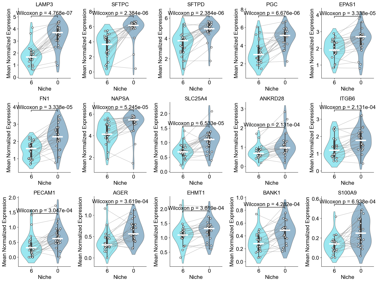
Transitional AT2
Compare Transitional AT2 cells between niche 6 (R2) and all other niches. For each slice, mean gene expression is calculated within niche 6 and outside niche 6, paired Wilcoxon tests are applied to determine which group has higher expression, and significant DEGs are identified after FDR correction.
[22]:
from scipy.stats import wilcoxon, mannwhitneyu
from statsmodels.stats.multitest import multipletests
from scipy.stats import rankdata
from statannotations.Annotator import Annotator
np.random.seed(1234)

noi_list = ['6', 'other']
ctoi = 'Transitional AT2'
min_cells = 20

qval_thres = 0.01
med_thres = 0

genes_list = cond_concat_new.var_names.tolist()
n_genes = len(genes_list)

avg_expr_noi1 = [[] for _ in range(n_genes)]
avg_expr_noi2 = [[] for _ in range(n_genes)]

for i, slice_name in enumerate(cond_name_list):

    adata = cond_concat_new[cond_concat_new.obs['slice_name'] == slice_name, :].copy()
    sc.pp.normalize_total(adata, target_sum=1e4)
    sc.pp.log1p(adata)

    adata_noi1 = adata[(adata.obs['final_CT'] == ctoi) & (adata.obs['niche_label'] == noi_list[0]), :].copy()
    adata_noi2 = adata[(adata.obs['final_CT'] == ctoi) & (adata.obs['niche_label'] != noi_list[0]), :].copy()

    n_cell_noi1 = adata_noi1.shape[0]
    n_cell_noi2 = adata_noi2.shape[0]

    if min(n_cell_noi1, n_cell_noi2) < min_cells:
        print(f"Skip {slice_name} due to rare cell count ({n_cell_noi1} vs {n_cell_noi2}).")
        continue

    for j, gene in enumerate(genes_list):
        avg_expr_noi1[j].append(np.mean(adata_noi1[:, gene].X))
        avg_expr_noi2[j].append(np.mean(adata_noi2[:, gene].X))

results = []
for j, gene in enumerate(genes_list):
    vals1 = np.array(avg_expr_noi1[j])
    vals2 = np.array(avg_expr_noi2[j])

    stat, pval = wilcoxon(vals1, vals2)

    diff = vals1 - vals2
    non_zero_mask = diff != 0
    diff_non_zero = diff[non_zero_mask]
    abs_diff = np.abs(diff_non_zero)
    ranks = rankdata(abs_diff)
    W_plus = np.sum(ranks[diff_non_zero > 0])
    W_minus = np.sum(ranks[diff_non_zero < 0])
    if W_plus > W_minus:
        greater=noi_list[0]
    else:
        greater=noi_list[1]

    results.append({
        'gene': gene,
        'stat': stat,
        'p-value': pval,
        'greater': greater,
        'median1': np.median(vals1),
        'median2': np.median(vals2),
        'median_max': max(np.median(vals1), np.median(vals2))
    })

df_results = pd.DataFrame(results)

df_results['q-value'] = multipletests(df_results['p-value'], method='fdr_bh')[1]

df_results['deg'] = 'FALSE'
# df_results.loc[(df_results['q-value'] < qval_thres) & (df_results['greater'] == noi_list[0]), 'deg'] = noi_list[0]
# df_results.loc[(df_results['q-value'] < qval_thres) & (df_results['greater'] == noi_list[1]), 'deg'] = noi_list[1]
df_results.loc[(df_results['q-value'] < qval_thres), 'deg'] = df_results.loc[(df_results['q-value'] < qval_thres) &
                                                                             (df_results['median_max'] > med_thres), 'greater']

df_deg_1 = df_results[df_results['deg'] == noi_list[0]].copy()
df_deg_1 = df_deg_1.sort_values('q-value', ascending=True)
df_deg_2 = df_results[df_results['deg'] == noi_list[1]].copy()
df_deg_2 = df_deg_2.sort_values('q-value', ascending=True)
Skip TILD049MA due to rare cell count (22 vs 4).
Skip TILD111LA due to rare cell count (1 vs 153).
Skip TILD113LA due to rare cell count (9 vs 96).
Skip VUILD102LA due to rare cell count (1 vs 145).
Skip VUILD102MA due to rare cell count (0 vs 197).
Skip VUILD105MA1 due to rare cell count (4 vs 228).
Skip VUILD105MA2 due to rare cell count (116 vs 15).
Skip VUILD142MA due to rare cell count (3 vs 22).
Skip VUILD48LA1 due to rare cell count (0 vs 361).
Skip VUILD48LA2 due to rare cell count (12 vs 552).
Skip VUILD49LA due to rare cell count (0 vs 215).
Skip VUILD91MA due to rare cell count (13 vs 218).
Skip VUILD96MA due to rare cell count (6 vs 11).
[23]:
np.random.seed(1234)

gene_list = df_deg_1['gene'].tolist()
print(gene_list)
n_genes = len(gene_list)

ncol = 5
nrow = int(np.ceil(n_genes / ncol))
fig, axes = plt.subplots(nrow, ncol, figsize=(3.2*ncol, 4*nrow))
axes = axes.flatten()

for j, gene in enumerate(gene_list):

    g_idx = df_results.index[df_results['gene'] == gene][0]

    vals1 = avg_expr_noi1[g_idx]
    vals2 = avg_expr_noi2[g_idx]
    ax = axes[j]

    df_plot = pd.DataFrame({
        'expr': np.concatenate([vals1, vals2]),
        'group': [noi_list[0]]*len(vals1)
               + [noi_list[1]]*len(vals2)
    })

    colors = [niche_color_dict[noi_list[0]], 'lightgray']
    sns.violinplot(x='group', y='expr', data=df_plot, ax=ax, palette=colors, cut=1, inner='box', width=0.8, alpha=0.5)

    for xpos, vals in zip([0,1],[vals1, vals2]):
        ax.hlines(np.median(vals), xpos-0.2, xpos+0.2,
                  color='white', lw=4, zorder=3)

    pairs = [(noi_list[0], noi_list[1])]
    annot = Annotator(ax, pairs, data=df_plot, x='group', y='expr')
    annot.configure(test='Wilcoxon', text_format='full', loc='inside', verbose=0, fontsize=16,)
    annot.apply_and_annotate()

    ax.set_title(gene, fontsize=14)
    ax.set_ylabel('mean normalized expression', fontsize=12)
    ax.set_xlabel('')
    ax.grid(False)
    for k in range(len(vals1)):
        jitter = 0.1
        xx1 = 0 + np.random.uniform(-jitter, jitter)
        xx2 = 1 + np.random.uniform(-jitter, jitter)
        ax.plot([xx1, xx2], [vals1[k], vals2[k]], color='gray', linewidth=1, alpha=0.5, zorder=1)
        ax.scatter(xx1, vals1[k], color='white', s=30, alpha=0.8, edgecolor='black', zorder=2)
        ax.scatter(xx2, vals2[k], color='white', s=30, alpha=0.8, edgecolor='black', zorder=2)

    ax.set_xticklabels([noi_list[0], noi_list[1]], fontsize=16)
    ax.tick_params(axis='y', labelsize=16)
    ax.set_title(gene, fontsize=16)
    ax.set_ylabel('Mean Normalized Expression', fontsize=16)
    ax.set_xlabel('Niche', fontsize=16)
    ax.grid(False)
    ax.spines['top'].set_visible(False)
    ax.spines['right'].set_visible(False)

for ax in axes[j+1:]:
    ax.axis('off')

print(f"{ctoi} (niche {noi_list[0]} vs niche {noi_list[1]})")
plt.tight_layout()
plt.show()
['SOX4', 'CEACAM5', 'CEACAM6', 'SCGB3A2', 'PDIA4', 'PDIA3', 'HSPA5', 'KRT5', 'ATP2A3', 'HES1', 'RNASE1', 'MMP7', 'STAT6', 'WFDC2', 'CTNNB1', 'WWTR1', 'ERN2', 'MGST1', 'NKX2-1', 'KRT17', 'IDH1', 'CST3', 'TTC19', 'SOX2', 'HLA-DRA', 'GSR', 'SPCS2', 'EHMT1', 'SOX9', 'PCNA', 'SOD2', 'XBP1', 'KIT', 'AXL', 'S100A2', 'MEG3', 'YAP1', 'HMGA1', 'EPCAM', 'UBE2J1', 'AKR1C1']
Transitional AT2 (niche 6 vs niche other)
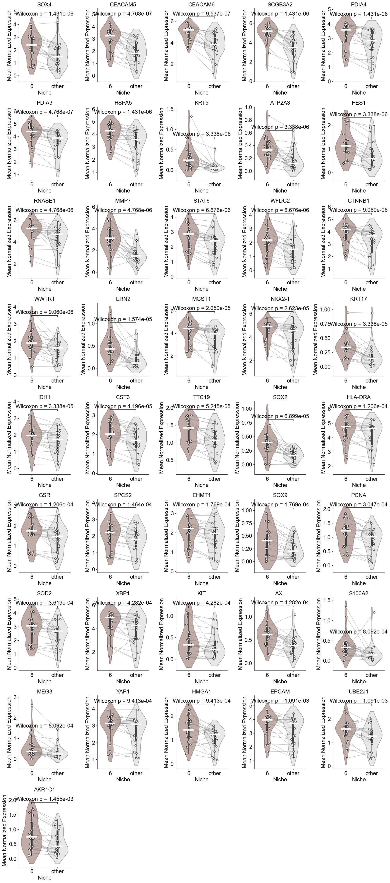
[24]:
np.random.seed(1234)

gene_list = df_deg_2['gene'].tolist()
print(gene_list)
n_genes = len(gene_list)

ncol = 5
nrow = int(np.ceil(n_genes / ncol))
fig, axes = plt.subplots(nrow, ncol, figsize=(3.2*ncol, 4*nrow))
axes = axes.flatten()

for j, gene in enumerate(gene_list):

    g_idx = df_results.index[df_results['gene'] == gene][0]

    vals1 = avg_expr_noi1[g_idx]
    vals2 = avg_expr_noi2[g_idx]
    ax = axes[j]

    df_plot = pd.DataFrame({
        'expr': np.concatenate([vals1, vals2]),
        'group': [noi_list[0]]*len(vals1)
               + [noi_list[1]]*len(vals2)
    })

    colors = [niche_color_dict[noi_list[0]], 'lightgray']
    sns.violinplot(x='group', y='expr', data=df_plot, ax=ax, palette=colors, cut=1, inner='box', width=0.8, alpha=0.5)

    for xpos, vals in zip([0,1],[vals1, vals2]):
        ax.hlines(np.median(vals), xpos-0.2, xpos+0.2,
                  color='white', lw=4, zorder=3)

    pairs = [(noi_list[0], noi_list[1])]
    annot = Annotator(ax, pairs, data=df_plot, x='group', y='expr')
    annot.configure(test='Wilcoxon', text_format='full', loc='inside', verbose=0, fontsize=16,)
    annot.apply_and_annotate()

    ax.set_title(gene, fontsize=14)
    ax.set_ylabel('mean normalized expression', fontsize=12)
    ax.set_xlabel('')
    ax.grid(False)
    for k in range(len(vals1)):
        jitter = 0.1
        xx1 = 0 + np.random.uniform(-jitter, jitter)
        xx2 = 1 + np.random.uniform(-jitter, jitter)
        ax.plot([xx1, xx2], [vals1[k], vals2[k]], color='gray', linewidth=1, alpha=0.5, zorder=1)
        ax.scatter(xx1, vals1[k], color='white', s=30, alpha=0.8, edgecolor='black', zorder=2)
        ax.scatter(xx2, vals2[k], color='white', s=30, alpha=0.8, edgecolor='black', zorder=2)

    ax.set_xticklabels([noi_list[0], noi_list[1]], fontsize=16)
    ax.tick_params(axis='y', labelsize=16)
    ax.set_title(gene, fontsize=16)
    ax.set_ylabel('Mean Normalized Expression', fontsize=16)
    ax.set_xlabel('Niche', fontsize=16)
    ax.spines['top'].set_visible(False)
    ax.spines['right'].set_visible(False)
    ax.grid(False)

for ax in axes[j+1:]:
    ax.axis('off')

print(f"{ctoi} (niche {noi_list[0]} vs niche {noi_list[1]})")
plt.tight_layout()
plt.show()
['SFTPC', 'FN1', 'LAMP3', 'PGC', 'PTGDS', 'SFTPD', 'SPARCL1', 'COL4A3', 'AGER', 'PECAM1', 'MCEMP1', 'LUM']
Transitional AT2 (niche 6 vs niche other)
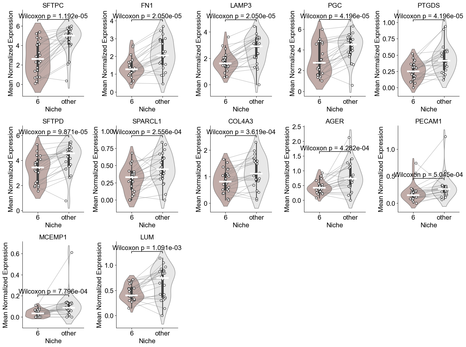
AT2 vs Transitional AT2
Compare AT2 and Transitional AT2 within niche 6 (R2). For each slice, compute mean gene expression for each cell type, perform paired Wilcoxon tests, determine which cell type shows higher expression, and identify significant DEGs after FDR correction.
[8]:
from scipy.stats import wilcoxon, mannwhitneyu
from statsmodels.stats.multitest import multipletests
from scipy.stats import rankdata
from statannotations.Annotator import Annotator
np.random.seed(1234)

noi = '6'
ctoi_list = ['Transitional AT2', 'AT2']
min_cells = 20

qval_thres = 0.01
med_thres = 1

genes_list = cond_concat_new.var_names.tolist()
n_genes = len(genes_list)

avg_expr_noi1 = [[] for _ in range(n_genes)]
avg_expr_noi2 = [[] for _ in range(n_genes)]

for i, slice_name in enumerate(cond_name_list):

    adata = cond_concat_new[cond_concat_new.obs['slice_name'] == slice_name, :].copy()
    sc.pp.normalize_total(adata, target_sum=1e4)
    sc.pp.log1p(adata)

    adata_noi1 = adata[(adata.obs['final_CT'] == ctoi_list[0]) & (adata.obs['niche_label'] == noi), :].copy()
    adata_noi2 = adata[(adata.obs['final_CT'] == ctoi_list[1]) & (adata.obs['niche_label'] == noi), :].copy()

    n_cell_noi1 = adata_noi1.shape[0]
    n_cell_noi2 = adata_noi2.shape[0]

    if min(n_cell_noi1, n_cell_noi2) < min_cells:
        print(f"Skip {slice_name} due to rare cell count ({n_cell_noi1} vs {n_cell_noi2}).")
        continue

    for j, gene in enumerate(genes_list):
        avg_expr_noi1[j].append(np.mean(adata_noi1[:, gene].X))
        avg_expr_noi2[j].append(np.mean(adata_noi2[:, gene].X))

results = []
for j, gene in enumerate(genes_list):
    vals1 = np.array(avg_expr_noi1[j])
    vals2 = np.array(avg_expr_noi2[j])

    stat, pval = wilcoxon(vals1, vals2)

    diff = vals1 - vals2
    non_zero_mask = diff != 0
    diff_non_zero = diff[non_zero_mask]
    abs_diff = np.abs(diff_non_zero)
    ranks = rankdata(abs_diff)
    W_plus = np.sum(ranks[diff_non_zero > 0])
    W_minus = np.sum(ranks[diff_non_zero < 0])
    if W_plus > W_minus:
        greater=ctoi_list[0]
    else:
        greater=ctoi_list[1]

    results.append({
        'gene': gene,
        'stat': stat,
        'p-value': pval,
        'greater': greater,
        'median1': np.median(vals1),
        'median2': np.median(vals2),
        'median_max': max(np.median(vals1), np.median(vals2))
    })

df_results = pd.DataFrame(results)

df_results['q-value'] = multipletests(df_results['p-value'], method='fdr_bh')[1]

df_results['deg'] = 'FALSE'
# df_results.loc[(df_results['q-value'] < qval_thres) & (df_results['greater'] == ctoi_list[0]), 'deg'] = ctoi_list[0]
# df_results.loc[(df_results['q-value'] < qval_thres) & (df_results['greater'] == ctoi_list[1]), 'deg'] = ctoi_list[1]
df_results.loc[(df_results['q-value'] < qval_thres), 'deg'] = df_results.loc[(df_results['q-value'] < qval_thres) &
                                                                             (df_results['median_max'] > med_thres), 'greater']

df_deg_1 = df_results[df_results['deg'] == ctoi_list[0]].copy()
df_deg_1 = df_deg_1.sort_values('q-value', ascending=True)
df_deg_2 = df_results[df_results['deg'] == ctoi_list[1]].copy()
df_deg_2 = df_deg_2.sort_values('q-value', ascending=True)
Skip TILD111LA due to rare cell count (1 vs 3).
Skip TILD113LA due to rare cell count (9 vs 21).
Skip VUILD102LA due to rare cell count (1 vs 0).
Skip VUILD102MA due to rare cell count (0 vs 0).
Skip VUILD105MA1 due to rare cell count (4 vs 7).
Skip VUILD142MA due to rare cell count (3 vs 39).
Skip VUILD48LA1 due to rare cell count (0 vs 4).
Skip VUILD48LA2 due to rare cell count (12 vs 21).
Skip VUILD49LA due to rare cell count (0 vs 2).
Skip VUILD91MA due to rare cell count (13 vs 11).
Skip VUILD96LA due to rare cell count (32 vs 18).
Skip VUILD96MA due to rare cell count (6 vs 7).
[9]:
np.random.seed(1234)

gene_list = df_deg_1['gene'].tolist()
print(gene_list)
n_genes = len(gene_list)

ncol = 5
nrow = int(np.ceil(n_genes / ncol))
fig, axes = plt.subplots(nrow, ncol, figsize=(3.2*ncol, 4*nrow))
axes = axes.flatten()

for j, gene in enumerate(gene_list):

    g_idx = df_results.index[df_results['gene'] == gene][0]

    vals1 = avg_expr_noi1[g_idx]
    vals2 = avg_expr_noi2[g_idx]
    ax = axes[j]

    df_plot = pd.DataFrame({
        'expr': np.concatenate([vals1, vals2]),
        'group': [ctoi_list[0]]*len(vals1)
               + [ctoi_list[1]]*len(vals2)
    })

    colors = [ct_color_dict[ctoi_list[0]], ct_color_dict[ctoi_list[1]]]
    sns.violinplot(x='group', y='expr', data=df_plot, ax=ax, palette=colors, cut=1, inner='box', width=0.8, alpha=0.5)

    for xpos, vals in zip([0,1],[vals1, vals2]):
        ax.hlines(np.median(vals), xpos-0.2, xpos+0.2,
                  color='white', lw=4, zorder=3)

    pairs = [(ctoi_list[0], ctoi_list[1])]
    annot = Annotator(ax, pairs, data=df_plot, x='group', y='expr')
    annot.configure(test='Wilcoxon', text_format='full', loc='inside', verbose=0, fontsize=16,)
    annot.apply_and_annotate()

    ax.set_title(gene, fontsize=14)
    ax.set_ylabel('mean normalized expression', fontsize=12)
    ax.set_xlabel('')
    ax.grid(False)
    for k in range(len(vals1)):
        jitter = 0.1
        xx1 = 0 + np.random.uniform(-jitter, jitter)
        xx2 = 1 + np.random.uniform(-jitter, jitter)
        ax.plot([xx1, xx2], [vals1[k], vals2[k]], color='gray', linewidth=1, alpha=0.5, zorder=1)
        ax.scatter(xx1, vals1[k], color='white', s=30, alpha=0.8, edgecolor='black', zorder=2)
        ax.scatter(xx2, vals2[k], color='white', s=30, alpha=0.8, edgecolor='black', zorder=2)

    ax.set_xticklabels([ctoi_list[0], ctoi_list[1]], fontsize=10)
    ax.tick_params(axis='y', labelsize=16)
    ax.set_title(gene, fontsize=16)
    ax.set_ylabel('Mean Normalized Expression', fontsize=16)
    ax.set_xlabel('Cell Type', fontsize=16)
    ax.grid(False)
    ax.spines['top'].set_visible(False)
    ax.spines['right'].set_visible(False)

for ax in axes[j+1:]:
    ax.axis('off')

print(f"({ctoi_list[0]} vs {ctoi_list[1]}) (niche {noi})")
plt.tight_layout()
plt.show()
['LMAN1', 'AGR3', 'MMP7', 'UBE2J1', 'ATG7', 'HLA-DQB1', 'PDIA4', 'BCL2L1', 'STAT6', 'CEACAM5', 'HES1', 'GSR', 'CTNNB1', 'VEGFA', 'SOX4', 'CST3', 'EPCAM', 'KRT15', 'TTC19', 'ANKRD28', 'SPCS2', 'EHMT1', 'NFKB1', 'NUCB2', 'SEC11C', 'TOP1', 'WWTR1', 'CEACAM6', 'AXIN2', 'HSPA5', 'MSLN', 'NUTF2', 'ERLEC1', 'MGST1', 'SELENOS', 'PKM', 'PCNA', 'STAT1', 'FKBP11', 'WFDC2', 'ITGA3', 'IDH1', 'CDH26', 'SSR3', 'PDIA6', 'NKX2-1', 'XBP1', 'ITGB6', 'SMAD4', 'DNAJB9', 'ITGB1', 'ITGAV', 'SPCS3', 'HYOU1', 'BAX', 'SFTA2', 'ATF4', 'PDIA3', 'FAS', 'DUOX1', 'MANF', 'EGFR', 'RHOA', 'SOD2', 'ICAM1', 'KRT18', 'EPAS1', 'HIF1A', 'HERPUD1', 'KRT8', 'YAP1', 'RNASE1', 'HIST1H1C', 'HMGA1', 'UCHL3', 'SCGB3A2', 'ACTA2', 'GKN2', 'PRDX4', 'COL1A1']
(Transitional AT2 vs AT2) (niche 6)
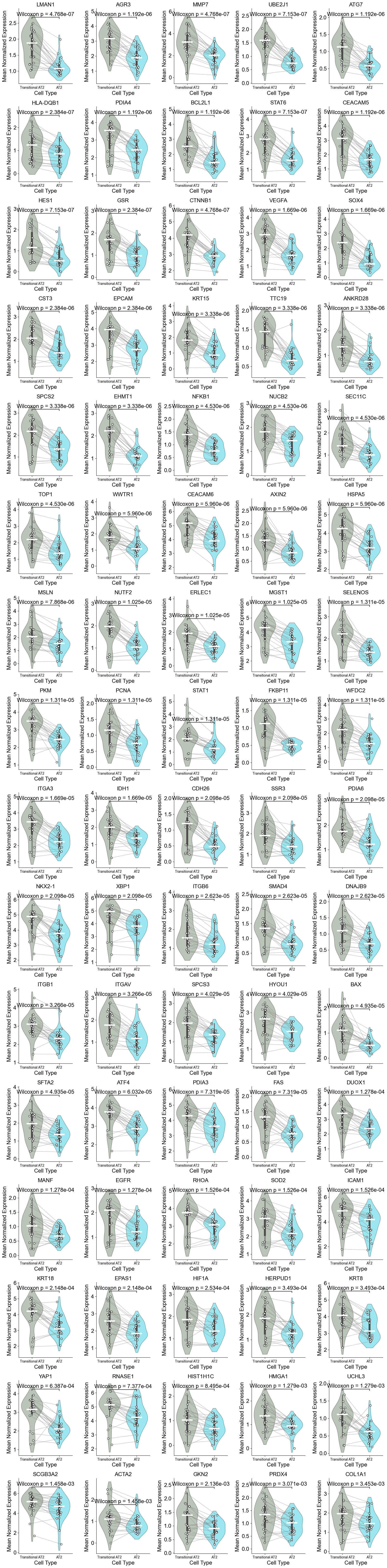
[11]:
np.random.seed(1234)

gene_list = df_deg_2['gene'].tolist()
print(gene_list)
n_genes = len(gene_list)

ncol = 5
nrow = int(np.ceil(n_genes / ncol))
fig, axes = plt.subplots(nrow, ncol, figsize=(3.2*ncol, 4*nrow))
axes = axes.flatten()

for j, gene in enumerate(gene_list):

    g_idx = df_results.index[df_results['gene'] == gene][0]

    vals1 = avg_expr_noi1[g_idx]
    vals2 = avg_expr_noi2[g_idx]
    ax = axes[j]

    df_plot = pd.DataFrame({
        'expr': np.concatenate([vals1, vals2]),
        'group': [ctoi_list[0]]*len(vals1)
               + [ctoi_list[1]]*len(vals2)
    })

    colors = [ct_color_dict[ctoi_list[0]], ct_color_dict[ctoi_list[1]]]
    sns.violinplot(x='group', y='expr', data=df_plot, ax=ax, palette=colors, cut=1, inner='box', width=0.8, alpha=0.5)

    for xpos, vals in zip([0,1],[vals1, vals2]):
        ax.hlines(np.median(vals), xpos-0.2, xpos+0.2,
                  color='white', lw=4, zorder=3)

    pairs = [(ctoi_list[0], ctoi_list[1])]
    annot = Annotator(ax, pairs, data=df_plot, x='group', y='expr')
    annot.configure(test='Wilcoxon', text_format='full', loc='inside', verbose=0, fontsize=16,)
    annot.apply_and_annotate()

    ax.set_title(gene, fontsize=14)
    ax.set_ylabel('mean normalized expression', fontsize=12)
    ax.set_xlabel('')
    ax.grid(False)
    for k in range(len(vals1)):
        jitter = 0.1
        xx1 = 0 + np.random.uniform(-jitter, jitter)
        xx2 = 1 + np.random.uniform(-jitter, jitter)
        ax.plot([xx1, xx2], [vals1[k], vals2[k]], color='gray', linewidth=1, alpha=0.5, zorder=1)
        ax.scatter(xx1, vals1[k], color='white', s=30, alpha=0.8, edgecolor='black', zorder=2)
        ax.scatter(xx2, vals2[k], color='white', s=30, alpha=0.8, edgecolor='black', zorder=2)

    ax.set_xticklabels([ctoi_list[0], ctoi_list[1]], fontsize=10)
    ax.tick_params(axis='y', labelsize=16)
    ax.set_title(gene, fontsize=16)
    ax.set_ylabel('Mean Normalized Expression', fontsize=16)
    ax.set_xlabel('Cell Type', fontsize=16)
    ax.spines['top'].set_visible(False)
    ax.spines['right'].set_visible(False)
    ax.grid(False)

for ax in axes[j+1:]:
    ax.axis('off')

print(f"({ctoi_list[0]} vs {ctoi_list[1]}) (niche {noi})")
plt.tight_layout()
plt.show()
['SFTPC', 'COL3A1', 'PGC']
(Transitional AT2 vs AT2) (niche 6)
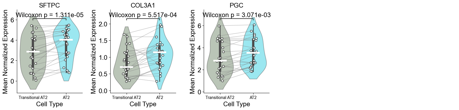
[72]:
adata_sub = cond_concat_new[(cond_concat_new.obs['final_CT'].isin(ctoi_list)) & (cond_concat_new.obs['niche_label'] == noi), :].copy()
sc.pp.normalize_total(adata_sub, target_sum=1e4)
sc.pp.log1p(adata_sub)
sc.tl.rank_genes_groups(adata_sub, groupby='final_CT', method="wilcoxon", pts=True)
res = adata_sub.uns["rank_genes_groups"]
[73]:
# logfc_cutoff = 0.2
# qval_cutoff = 0.05
# pts_cutoff = 0.3
# top_n = 5

# top_genes_by_ct_4wk = {}
# for ct in ctoi_list:
#     genes = pd.Index(res["names"][ct], name="gene")
#     pts_series = res["pts"][ct]
#     pts_aligned = pts_series.reindex(genes)
#     df = pd.DataFrame({
#         "gene": res["names"][ct],
#         "logFC": res["logfoldchanges"][ct],
#         "qval": res["pvals_adj"][ct],
#         "score": res["scores"][ct],
#         "pts": pts_aligned.values,
#     })
#     df = df[(df["qval"] < qval_cutoff) & (df["logFC"] > logfc_cutoff) & (df["pts"] > pts_cutoff)]
#     df = df.sort_values("logFC", ascending=False)
#     top_genes_by_ct_4wk[ct] = df["gene"].head(top_n).tolist()

# gene_list = []
# seen = set()
# for ct in ctoi_list:
#     for g in top_genes_by_ct_4wk[ct]:
#         if g not in seen:
#             gene_list.append(g)
#             seen.add(g)

gene_list = ['CEACAM5', 'MMP7', 'WFDC2', 'STAT1', 'VEGFA', 'SOX4', 'KRT8', 'SFTPC', 'PGC', 'DMBT1']

fig, ax = plt.subplots(figsize=(5.5, 4))

sc.pl.dotplot(
    adata_sub,
    var_names=gene_list,
    groupby="final_CT",
    # standard_scale="var",
    dot_max=0.6,
    ax=ax,
    show=False,
    # cmap="RdBu_r",
)

ax.set_title("AT2 vs Transitional AT2", fontsize=16)
plt.tight_layout()
plt.show()
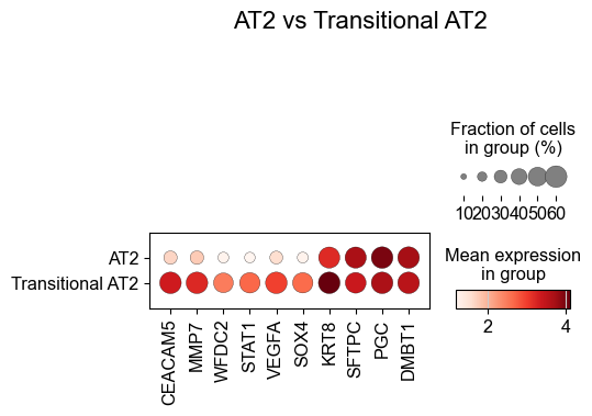
The fraction of AGER+ cells
[74]:
import numpy as np
import scipy.sparse as sp

X = adata_sub[:, 'AGER'].X

if sp.issparse(X):
    ager = X.toarray().ravel()
else:
    ager = X.ravel()

ct = adata_sub.obs['final_CT'].astype(str).values

mask_at2 = (ct == 'AT2')
mask_trans = (ct == 'Transitional AT2')

prop_at2 = np.mean(ager[mask_at2] > 0)
prop_trans = np.mean(ager[mask_trans] > 0)

# print("AT2 AGER+ proportion:", prop_at2)
# print("Transitional AT2 AGER+ proportion:", prop_trans)

df = pd.DataFrame({
    "Cell type": ["AT2", "Transitional AT2"],
    "AGER+ proportion": [prop_at2, prop_trans]
})

palette = [ct_color_dict["AT2"], ct_color_dict["Transitional AT2"]]

fig, ax = plt.subplots(figsize=(3, 4))

sns.barplot(data=df, x="Cell type", y="AGER+ proportion", palette=palette, ax=ax, width=0.7, alpha=0.8)

for p in ax.patches:
    h = p.get_height()
    ax.text(p.get_x() + p.get_width() / 2, h, f"{h:.3f}", ha="center", va="bottom", fontsize=16)

ax.set_ylabel(None)
ax.set_xlabel(None)
ax.tick_params(axis='x', labelsize=14)
ax.tick_params(axis='y', labelsize=16)
ax.set_title("AGER+ proportion", fontsize=16, pad=10)
ax.grid(False)
ax.spines['top'].set_visible(False)
ax.spines['right'].set_visible(False)

plt.tight_layout()
plt.show()
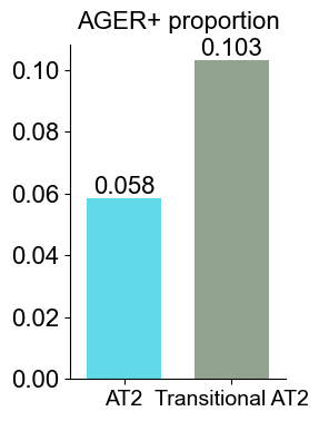
AT2 (3 niches)
Compare AT2 cells across three niches (0, 5, and 6) by calculating mean expression of selected genes in each niche for every slice, visualizing the distributions with violin plots, marking median values, connecting paired observations across niches, and performing pairwise Wilcoxon tests to assess statistical differences.
[26]:
from scipy.stats import wilcoxon, mannwhitneyu
from statsmodels.stats.multitest import multipletests
from scipy.stats import rankdata
from statannotations.Annotator import Annotator
np.random.seed(1234)

noi_list = ['0', '5', '6']
ctoi = 'AT2'
min_cells = 20

gene_list1 = ['CEACAM6', 'KRT17', 'MMP7', 'KRT15', 'SCGB3A2', 'SCGB1A1', 'CEACAM5', 'SOX4', 'WFDC2', 'SFTPC', 'SFTPD', 'NAPSA', 'LAMP3']

# qval_thres = 0.01

n_genes = len(gene_list1)

avg_expr_noi1 = [[] for _ in range(n_genes)]
avg_expr_noi2 = [[] for _ in range(n_genes)]
avg_expr_noi3 = [[] for _ in range(n_genes)]

for i, slice_name in enumerate(cond_name_list):

    adata = cond_concat_new[cond_concat_new.obs['slice_name'] == slice_name, :].copy()
    sc.pp.normalize_total(adata, target_sum=1e4)
    sc.pp.log1p(adata)

    adata_noi1 = adata[(adata.obs['final_CT'] == ctoi) & (adata.obs['niche_label'] == noi_list[0]), :].copy()
    adata_noi2 = adata[(adata.obs['final_CT'] == ctoi) & (adata.obs['niche_label'] == noi_list[1]), :].copy()
    adata_noi3 = adata[(adata.obs['final_CT'] == ctoi) & (adata.obs['niche_label'] == noi_list[2]), :].copy()

    n_cell_noi1 = adata_noi1.shape[0]
    n_cell_noi2 = adata_noi2.shape[0]
    n_cell_noi3 = adata_noi3.shape[0]

    if min(n_cell_noi1, n_cell_noi2, n_cell_noi3) < min_cells:
        print(f"Skip {slice_name} due to rare cell count ({n_cell_noi1} vs {n_cell_noi2} vs {n_cell_noi3}).")
        continue

    for j, gene in enumerate(gene_list1):
        avg_expr_noi1[j].append(np.mean(adata_noi1[:, gene].X))
        avg_expr_noi2[j].append(np.mean(adata_noi2[:, gene].X))
        avg_expr_noi3[j].append(np.mean(adata_noi3[:, gene].X))

ncol = 5
nrow = int(np.ceil(n_genes / ncol))
fig, axes = plt.subplots(nrow, ncol, figsize=(4*ncol, 4*nrow))
axes = axes.flatten()

for j, gene in enumerate(gene_list1):
    vals1 = avg_expr_noi1[j]
    vals2 = avg_expr_noi2[j]
    vals3 = avg_expr_noi3[j]
    ax = axes[j]

    df_plot = pd.DataFrame({
        'expr': np.concatenate([vals1, vals2, vals3]),
        'group': [noi_list[0]]*len(vals1)
               + [noi_list[1]]*len(vals2)
               + [noi_list[2]]*len(vals3)
    })

    colors = [niche_color_dict[noi_list[0]], niche_color_dict[noi_list[1]], niche_color_dict[noi_list[2]]]
    sns.violinplot(x="group", y="expr", data=df_plot, ax=ax, palette=colors, cut=1, inner='box', alpha=0.5)

    for xpos, vals in zip([0,1,2],[vals1, vals2, vals3]):
        ax.hlines(np.median(vals), xpos-0.2, xpos+0.2,
                  color='white', lw=4, zorder=3)

    pairs = [(noi_list[0], noi_list[1]), (noi_list[1], noi_list[2]), (noi_list[0], noi_list[2])]
    annot = Annotator(ax, pairs, data=df_plot, x='group', y='expr')
    annot.configure(test='Wilcoxon', text_format='full', loc='inside', verbose=0, fontsize=16,)
    annot.apply_and_annotate()

    ax.set_title(gene, fontsize=14)
    ax.set_ylabel('mean scaled expression', fontsize=12)
    ax.set_xlabel('')
    ax.grid(False)
    for k in range(len(vals1)):
        jitter = 0.1
        xx1 = 0 + np.random.uniform(-jitter, jitter)
        xx2 = 1 + np.random.uniform(-jitter, jitter)
        xx3 = 2 + np.random.uniform(-jitter, jitter)
        ax.plot([xx1, xx2], [vals1[k], vals2[k]], color="gray", linewidth=1, alpha=0.5, zorder=1)
        ax.plot([xx2, xx3], [vals2[k], vals3[k]], color="gray", linewidth=1, alpha=0.5, zorder=1)
        ax.scatter(xx1, vals1[k], color='white', s=30, alpha=0.8, edgecolor="black", zorder=2)
        ax.scatter(xx2, vals2[k], color='white', s=30, alpha=0.8, edgecolor="black", zorder=2)
        ax.scatter(xx3, vals3[k], color='white', s=30, alpha=0.8, edgecolor="black", zorder=2)

    ax.set_xticklabels([noi_list[0], noi_list[1], noi_list[2]], fontsize=16)
    ax.tick_params(axis='y', labelsize=16)
    ax.set_title(gene, fontsize=16)
    ax.set_ylabel('Mean Normalized Expression', fontsize=16)
    ax.set_xlabel('Niche', fontsize=16)
    ax.spines['top'].set_visible(False)
    ax.spines['right'].set_visible(False)
    ax.grid(False)

for ax in axes[n_genes:]:
    ax.axis('off')

plt.suptitle(f"{ctoi} (niche {noi_list[0]} vs niche {noi_list[1]} vs niche {noi_list[2]})", fontsize=20)
plt.tight_layout()
plt.show()
Skip TILD049MA due to rare cell count (1 vs 5 vs 30).
Skip TILD111LA due to rare cell count (1066 vs 186 vs 3).
Skip TILD117MA2 due to rare cell count (16 vs 164 vs 626).
Skip TILD175MA due to rare cell count (15 vs 50 vs 182).
Skip VUILD102LA due to rare cell count (2702 vs 648 vs 0).
Skip VUILD102MA due to rare cell count (1641 vs 1475 vs 0).
Skip VUILD105MA1 due to rare cell count (140 vs 226 vs 7).
Skip VUILD105MA2 due to rare cell count (0 vs 29 vs 156).
Skip VUILD48LA1 due to rare cell count (987 vs 667 vs 4).
Skip VUILD49LA due to rare cell count (638 vs 1180 vs 2).
Skip VUILD91MA due to rare cell count (432 vs 926 vs 11).
Skip VUILD96LA due to rare cell count (2890 vs 270 vs 18).
Skip VUILD96MA due to rare cell count (0 vs 1 vs 7).
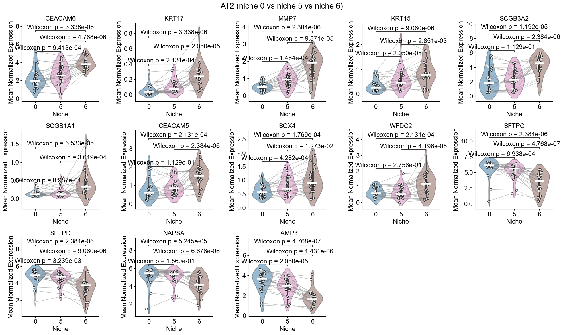
Disease progression
All CSNs
Assess the relationship between pathology and CSN proportion by calculating the Pearson correlation across slices, performing a permutation test with 10,000 random shuffles to evaluate significance, and visualizing both the observed correlation with a regression line and the null distribution of permuted correlations.
[27]:
from scipy.stats import pearsonr, spearmanr

n_permutations = 10000
np.random.seed(1234)

patho_annot = []
niche_prop = []
for i, slice_name in enumerate(cond_name_list):

    adata = cond_concat_new[cond_concat_new.obs['slice_name'] == slice_name, :].copy()

    patho_annot.append(adata.obs['percent_pathology'][0])
    niche_prop.append(np.mean(adata.obs['csn_label'] != 'basic'))

patho_annot = np.array(patho_annot) / 100
niche_prop  = np.array(niche_prop)

obs_r, _ = pearsonr(patho_annot, niche_prop)

perm_rs = np.zeros(n_permutations)
for i in range(n_permutations):
    permuted = np.random.permutation(niche_prop)
    perm_rs[i], _ = pearsonr(patho_annot, permuted)

p_perm = np.mean(np.abs(perm_rs) >= np.abs(obs_r))

fig, axes = plt.subplots(1, 2, figsize=(12, 5))

axes[0].scatter(patho_annot, niche_prop, color='royalblue', s=40, alpha=0.7)
m, b = np.polyfit(patho_annot, niche_prop, 1)
x_line = np.linspace(min(patho_annot), max(patho_annot), 100)
y_line = m * x_line + b
axes[0].plot(x_line, y_line,  color='gray', linewidth=3)
axes[0].set_title(f'Observed correlation\n$r$ = {obs_r:.2f}  $p$ = {p_perm:.4f}', fontsize=16)
axes[0].set_xlabel('Percent Pathology', fontsize=16)
axes[0].set_ylabel('CSN Proportion', fontsize=16)
axes[0].spines['top'].set_visible(False)
axes[0].spines['right'].set_visible(False)
axes[0].grid(False)

axes[1].hist(perm_rs, bins=50, color='royalblue', edgecolor='black', alpha=0.7)
axes[1].axvline(obs_r, linestyle='--', color='red', linewidth=2, label=f'Observed $r$ = {obs_r:.2f}')
axes[1].axvline(-obs_r, linestyle='--', color='red', linewidth=2)
axes[1].set_title(f'Permutation Test\n$p$ = {p_perm:.4f}', fontsize=16)
axes[1].set_xlabel("Permuted Pearson's $r$", fontsize=16)
axes[1].set_ylabel('Frequency', fontsize=16)
axes[1].spines['top'].set_visible(False)
axes[1].spines['right'].set_visible(False)
axes[1].grid(False)
axes[1].legend(fontsize=14)

plt.tight_layout()
plt.show()
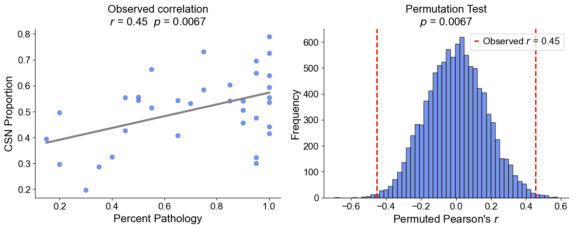
Individual niche
Quantify the association between percent pathology and the proportion of each niche across slices by computing Pearson correlations, performing 10,000-permutation tests to assess significance, and visualizing for each niche both the scatter plot with regression line and the null distribution of permuted correlations.
[28]:
n_permutations = 10000
np.random.seed(1234)

n_niche = len(cond_concat_new.uns['niche_label_summary'])
fig, axes = plt.subplots(n_niche, 2, figsize=(12, 5*n_niche))
axes = axes.flatten()

for j, niche in enumerate(cond_concat_new.uns['niche_label_summary']):
    patho_annot = []
    niche_prop = []
    for i, slice_name in enumerate(cond_name_list):

        adata = cond_concat_new[cond_concat_new.obs['slice_name'] == slice_name, :].copy()

        patho_annot.append(adata.obs['percent_pathology'][0])
        niche_prop.append(np.mean(adata.obs['niche_label'] == niche))

    patho_annot = np.array(patho_annot) / 100
    niche_prop  = np.array(niche_prop)

    obs_r, _ = pearsonr(patho_annot, niche_prop)

    perm_rs = np.zeros(n_permutations)
    for i in range(n_permutations):
        permuted = np.random.permutation(niche_prop)
        perm_rs[i], _ = pearsonr(patho_annot, permuted)

    p_perm = np.mean(np.abs(perm_rs) >= np.abs(obs_r))

    axes[2*j].scatter(patho_annot, niche_prop, color=niche_color_dict[niche], s=40, alpha=0.7)
    m, b = np.polyfit(patho_annot, niche_prop, 1)
    x_line = np.linspace(min(patho_annot), max(patho_annot), 100)
    y_line = m * x_line + b
    axes[2*j].plot(x_line, y_line,  color='gray', linewidth=3)
    axes[2*j].set_title(f'Observed correlation\n$r$ = {obs_r:.2f}  $p$ = {p_perm:.4f}', fontsize=16)
    axes[2*j].set_xlabel('Percent Pathology', fontsize=16)
    axes[2*j].set_ylabel(f'Niche {niche} Proportion', fontsize=16)
    axes[2*j].spines['top'].set_visible(False)
    axes[2*j].spines['right'].set_visible(False)
    axes[2*j].grid(False)

    axes[1+2*j].hist(perm_rs, bins=50, color=niche_color_dict[niche], edgecolor='black', alpha=0.7)
    axes[1+2*j].axvline(obs_r, linestyle='--', color='red', linewidth=2, label=f'Observed $r$ = {obs_r:.2f}')
    axes[1+2*j].axvline(-obs_r, linestyle='--', color='red', linewidth=2)
    axes[1+2*j].set_title(f'Permutation Test\n$p$ = {p_perm:.4f}', fontsize=16)
    axes[1+2*j].set_xlabel("Permuted Pearson's $r$", fontsize=16)
    axes[1+2*j].set_ylabel('Frequency', fontsize=16)
    axes[1+2*j].spines['top'].set_visible(False)
    axes[1+2*j].spines['right'].set_visible(False)
    axes[1+2*j].grid(False)
    axes[1+2*j].legend(fontsize=14)

plt.tight_layout()
plt.show()
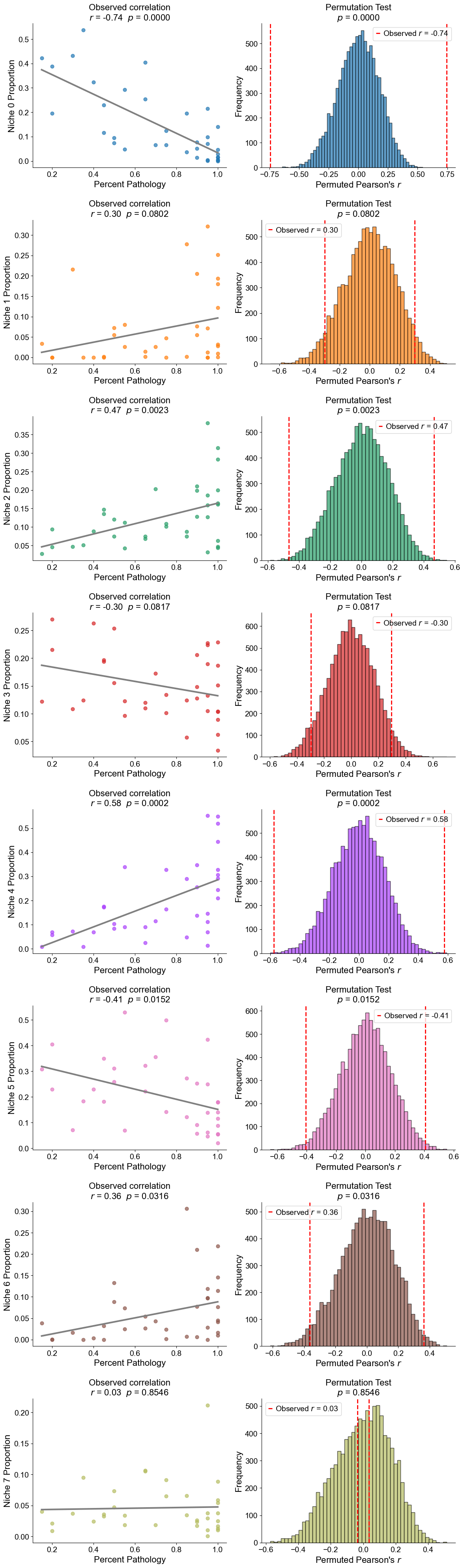
Celltype proportion within niches
Quantify the association between percent pathology and the proportion of each cell type within a given niche as well as across whole slices by computing Pearson correlations, performing 10,000-permutation tests to assess significance, and visualizing for each cell type in a 4-panel layout: scatter plot with regression line and permutation histogram for both the niche-specific and whole-slice proportions.
[29]:
from scipy.stats import pearsonr, spearmanr
n_permutations = 10000
np.random.seed(1234)

# niche = '4'
for niche in cond_concat_new.uns['niche_label_summary']:

    print(f'Niche {niche}: {niche_annot[niche]}')

    enr_ct_list = enr_result[niche]

    n_ct = len(enr_ct_list)
    fig, axes = plt.subplots(n_ct, 4, figsize=(24, 5*n_ct))
    axes = axes.flatten()

    for j, ct in enumerate(enr_ct_list):
        patho_annot = []
        ct_prop = []
        for i, slice_name in enumerate(cond_name_list):

            adata = cond_concat_new[(cond_concat_new.obs['slice_name'] == slice_name) & (cond_concat_new.obs['niche_label'] == niche), :].copy()
            if adata.shape[0] == 0:
                continue

            patho_annot.append(adata.obs['percent_pathology'][0])
            ct_prop.append(np.mean(adata.obs['final_CT'] == ct))

        patho_annot = np.array(patho_annot) / 100
        ct_prop  = np.array(ct_prop)

        obs_r, _ = pearsonr(patho_annot, ct_prop)

        perm_rs = np.zeros(n_permutations)
        for i in range(n_permutations):
            permuted = np.random.permutation(ct_prop)
            perm_rs[i], _ = pearsonr(patho_annot, permuted)

        p_perm = np.mean(np.abs(perm_rs) >= np.abs(obs_r))

        axes[4*j].scatter(patho_annot, ct_prop, color=ct_color_dict[ct], s=40, alpha=0.7)
        m, b = np.polyfit(patho_annot, ct_prop, 1)
        x_line = np.linspace(min(patho_annot), max(patho_annot), 100)
        y_line = m * x_line + b
        axes[4*j].plot(x_line, y_line,  color='gray', linewidth=3)
        axes[4*j].set_title(f'Observed correlation\n$r$ = {obs_r:.2f}  $p$ = {p_perm:.4f}', fontsize=16)
        axes[4*j].set_xlabel('Percent Pathology', fontsize=16)
        axes[4*j].set_ylabel(f'Proportion of {ct}\nNiche {niche}', fontsize=16)
        axes[4*j].spines['top'].set_visible(False)
        axes[4*j].spines['right'].set_visible(False)
        axes[4*j].grid(False)

        axes[1+4*j].hist(perm_rs, bins=50, color=ct_color_dict[ct], edgecolor='black', alpha=0.7)
        axes[1+4*j].axvline(obs_r, linestyle='--', color='red', linewidth=2, label=f'Observed $r$ = {obs_r:.2f}')
        axes[1+4*j].axvline(-obs_r, linestyle='--', color='red', linewidth=2)
        axes[1+4*j].set_title(f'Permutation Test\n$p$ = {p_perm:.4f}', fontsize=16)
        axes[1+4*j].set_xlabel("Permuted Pearson's $r$", fontsize=16)
        axes[1+4*j].set_ylabel('Frequency', fontsize=16)
        axes[1+4*j].spines['top'].set_visible(False)
        axes[1+4*j].spines['right'].set_visible(False)
        axes[1+4*j].grid(False)
        axes[1+4*j].legend(fontsize=14)

        patho_annot = []
        ct_prop = []
        for i, slice_name in enumerate(cond_name_list):

            adata = cond_concat_new[(cond_concat_new.obs['slice_name'] == slice_name), :].copy()
            if adata.shape[0] == 0:
                print(f'Skipping {slice_name}.')
                continue

            patho_annot.append(adata.obs['percent_pathology'][0])
            ct_prop.append(np.mean(adata.obs['final_CT'] == ct))

        patho_annot = np.array(patho_annot) / 100
        ct_prop  = np.array(ct_prop)

        obs_r, _ = pearsonr(patho_annot, ct_prop)

        perm_rs = np.zeros(n_permutations)
        for i in range(n_permutations):
            permuted = np.random.permutation(ct_prop)
            perm_rs[i], _ = pearsonr(patho_annot, permuted)

        p_perm = np.mean(np.abs(perm_rs) >= np.abs(obs_r))

        axes[2+4*j].scatter(patho_annot, ct_prop, color=ct_color_dict[ct], s=40, alpha=0.7)
        m, b = np.polyfit(patho_annot, ct_prop, 1)
        x_line = np.linspace(min(patho_annot), max(patho_annot), 100)
        y_line = m * x_line + b
        axes[2+4*j].plot(x_line, y_line,  color='gray', linewidth=3)
        axes[2+4*j].set_title(f'Observed correlation\n$r$ = {obs_r:.2f}  $p$ = {p_perm:.4f}', fontsize=16)
        axes[2+4*j].set_xlabel('Percent Pathology', fontsize=16)
        axes[2+4*j].set_ylabel(f'Proportion of {ct}\nWhole slice', fontsize=16)
        axes[2+4*j].spines['top'].set_visible(False)
        axes[2+4*j].spines['right'].set_visible(False)
        axes[2+4*j].grid(False)

        axes[3+4*j].hist(perm_rs, bins=50, color=ct_color_dict[ct], edgecolor='black', alpha=0.7)
        axes[3+4*j].axvline(obs_r, linestyle='--', color='red', linewidth=2, label=f'Observed $r$ = {obs_r:.2f}')
        axes[3+4*j].axvline(-obs_r, linestyle='--', color='red', linewidth=2)
        axes[3+4*j].set_title(f'Permutation Test\n$p$ = {p_perm:.4f}', fontsize=16)
        axes[3+4*j].set_xlabel("Permuted Pearson's $r$", fontsize=16)
        axes[3+4*j].set_ylabel('Frequency', fontsize=16)
        axes[3+4*j].spines['top'].set_visible(False)
        axes[3+4*j].spines['right'].set_visible(False)
        axes[3+4*j].grid(False)
        axes[3+4*j].legend(fontsize=14)

    plt.tight_layout()
    plt.show()
Niche 0: Alveolar epithelium
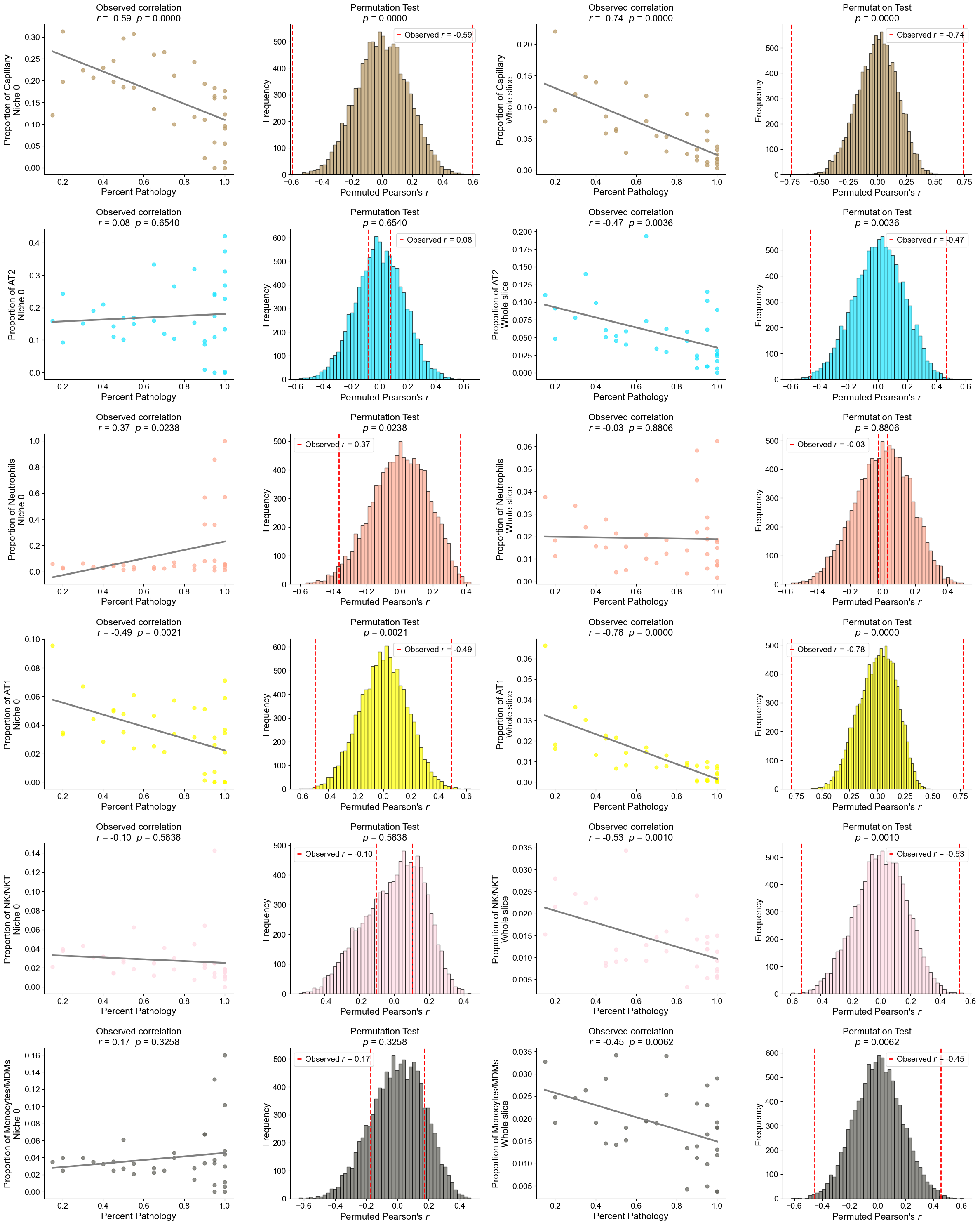
Niche 1: Airway epithelium
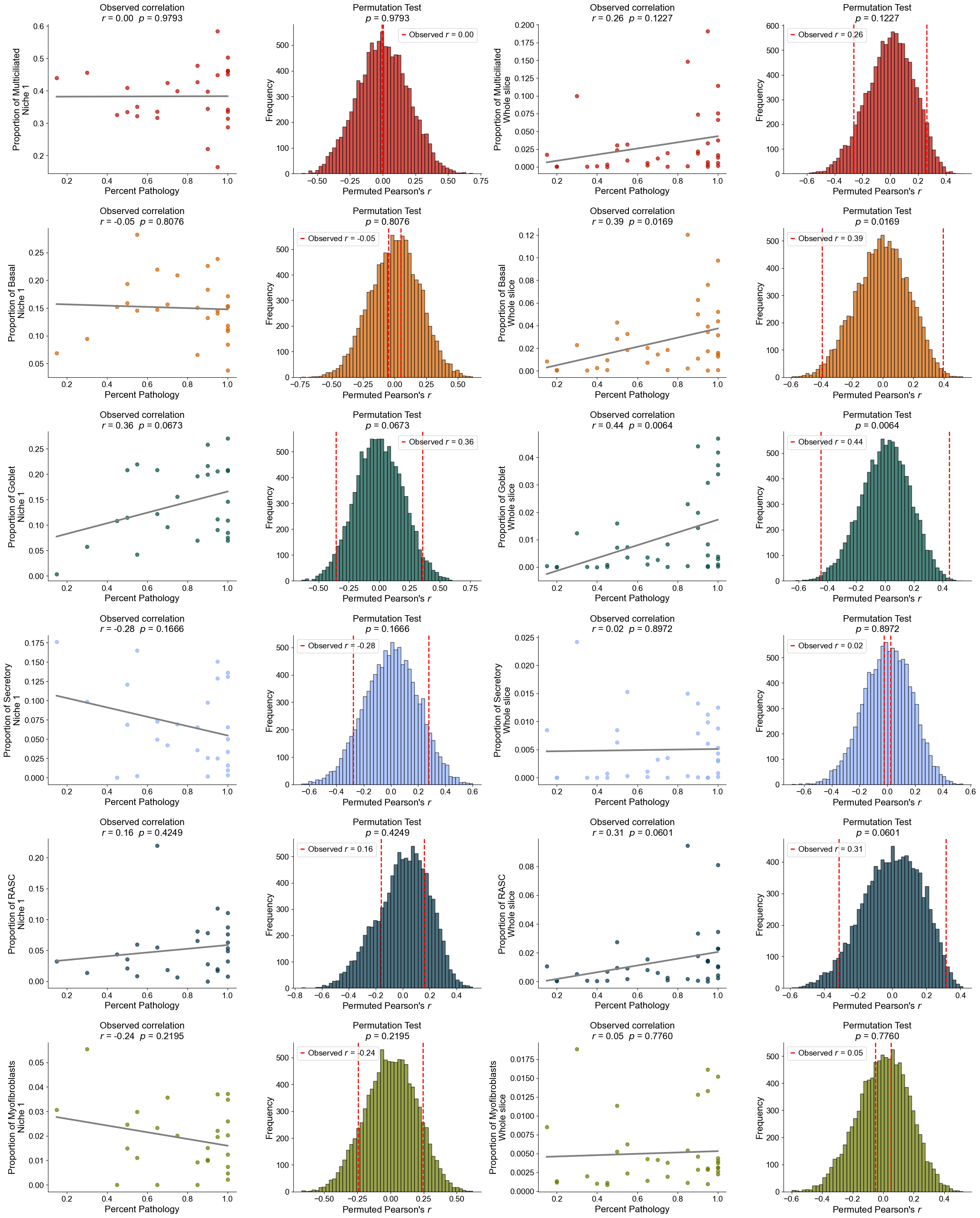
Niche 2: Interstitial fibrotic
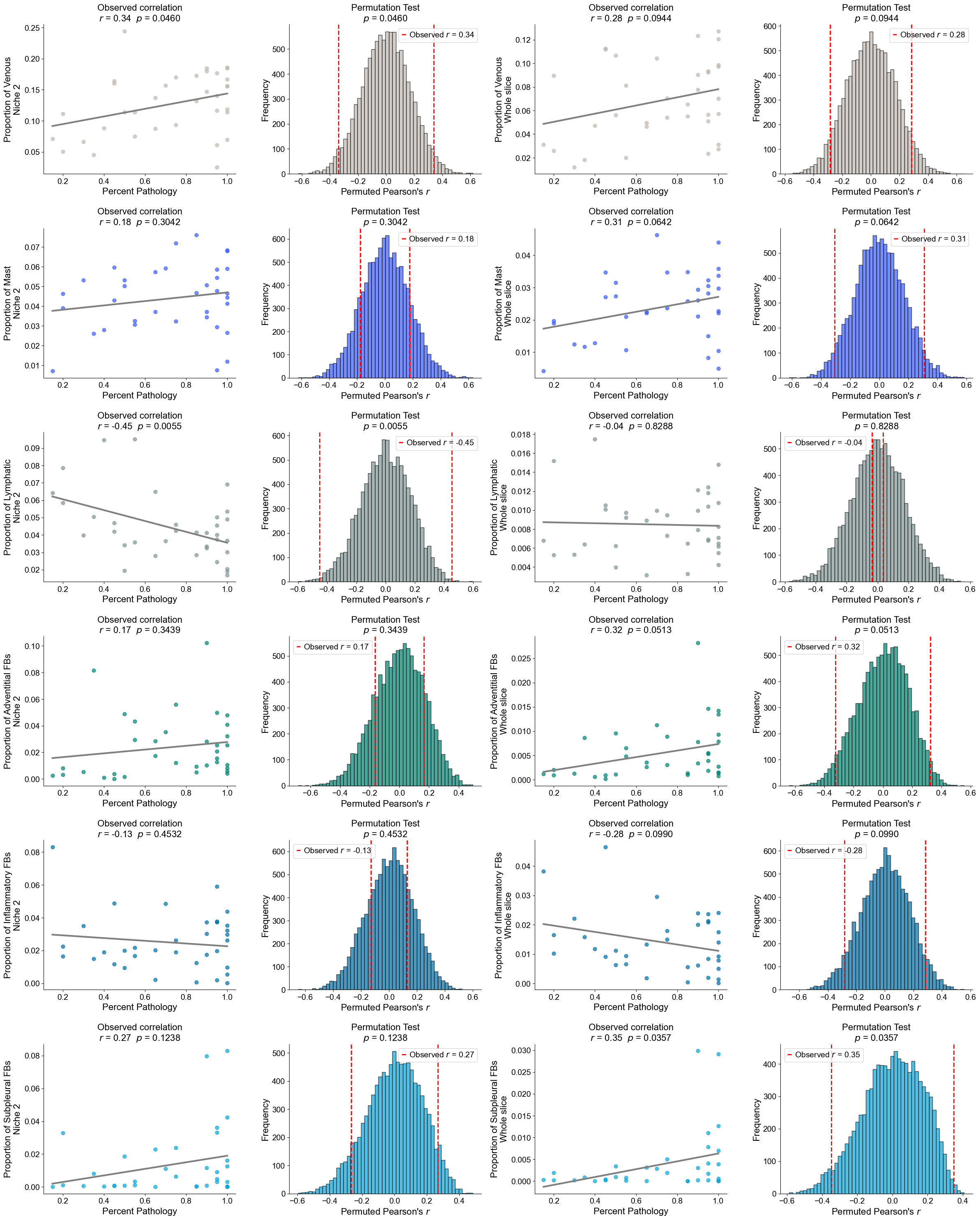
Niche 3: Vascular
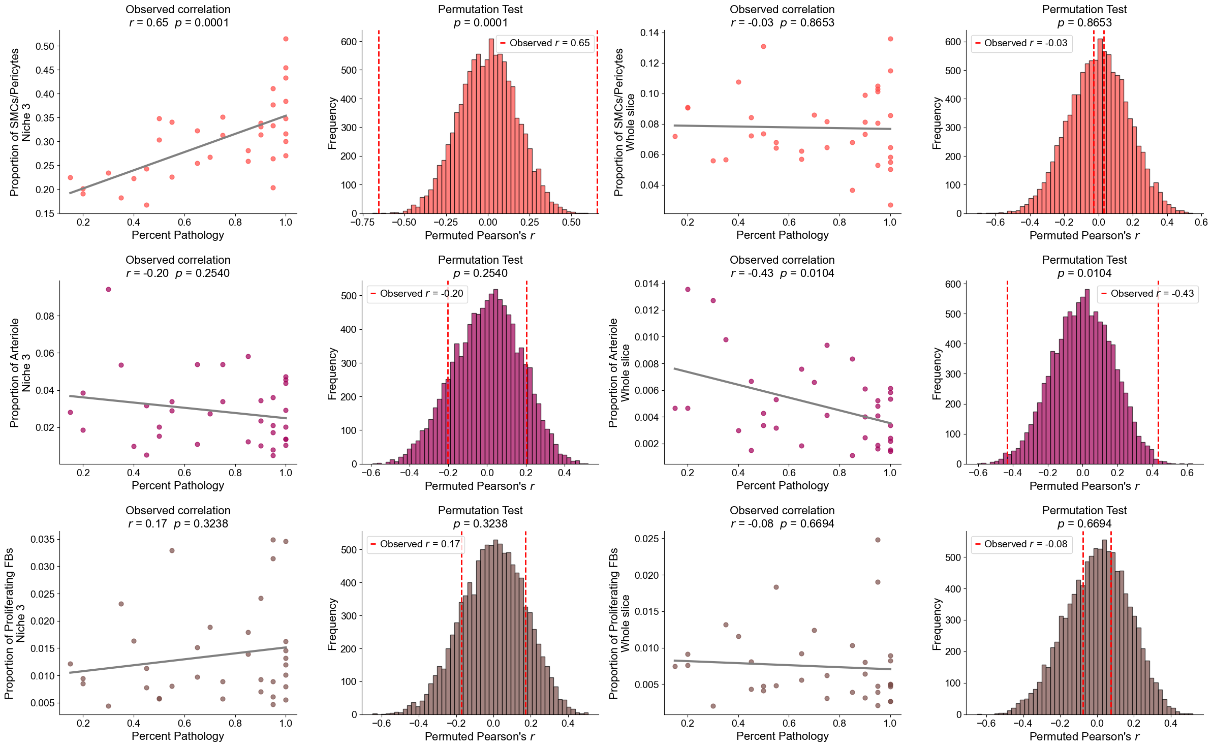
Niche 4: Lymphoid immune aggregates
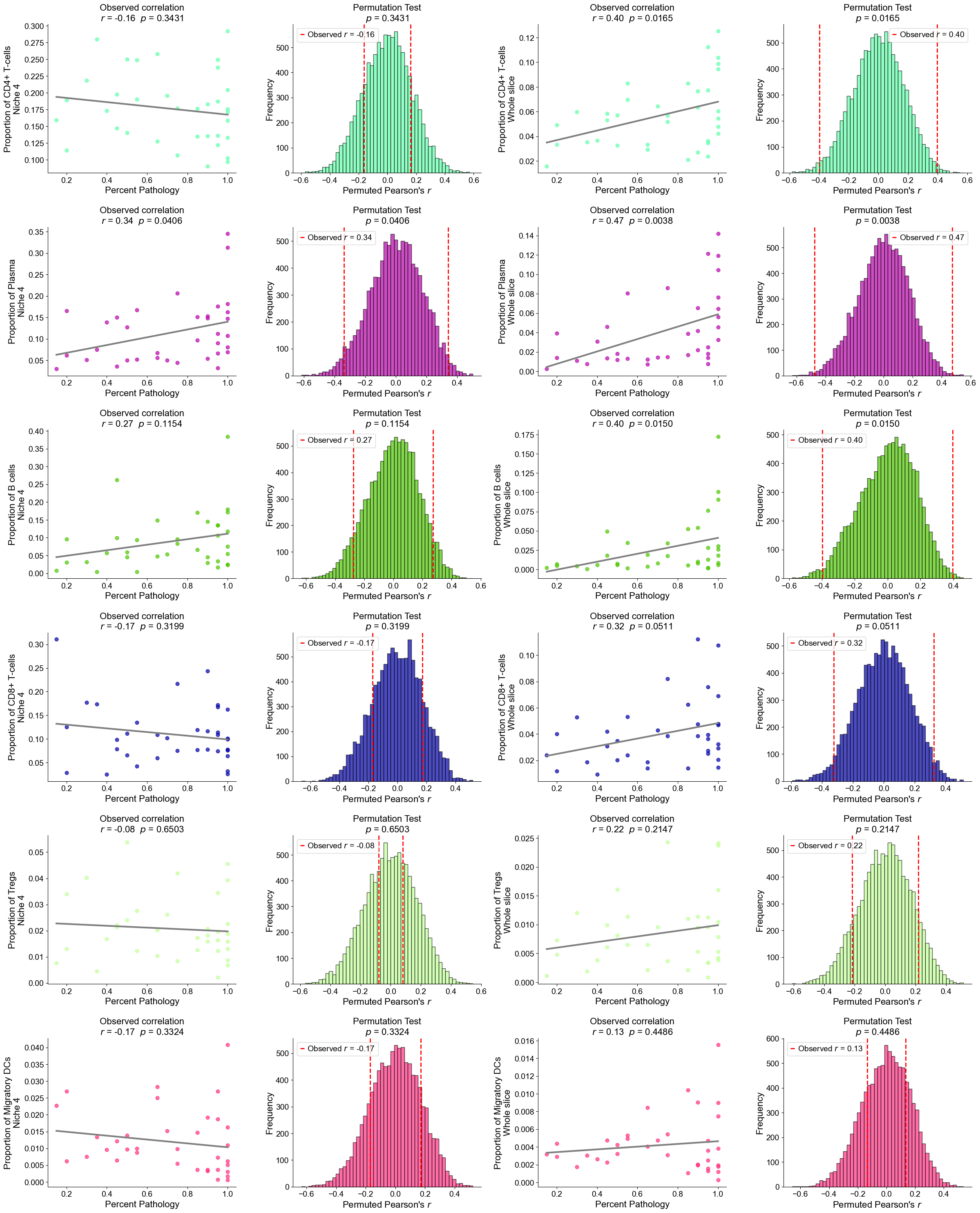
Niche 5: Fibrotic foci
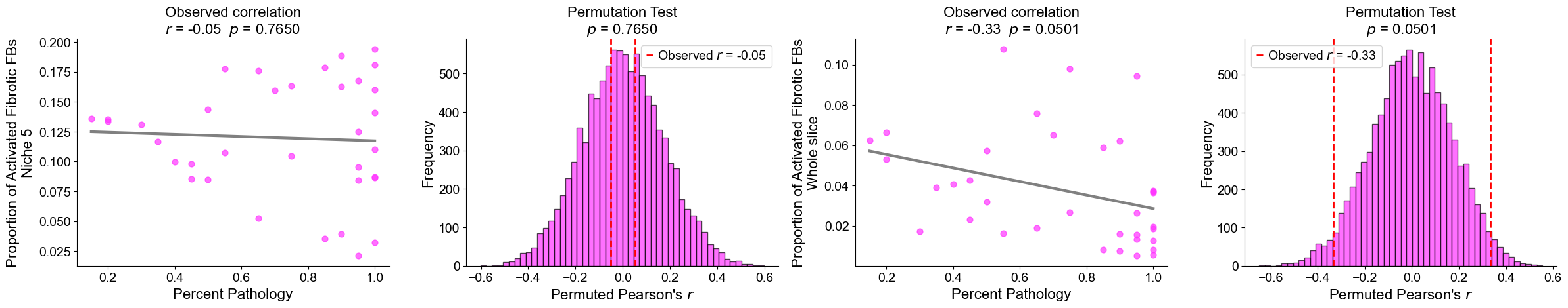
Niche 6: Aberrant epithelium
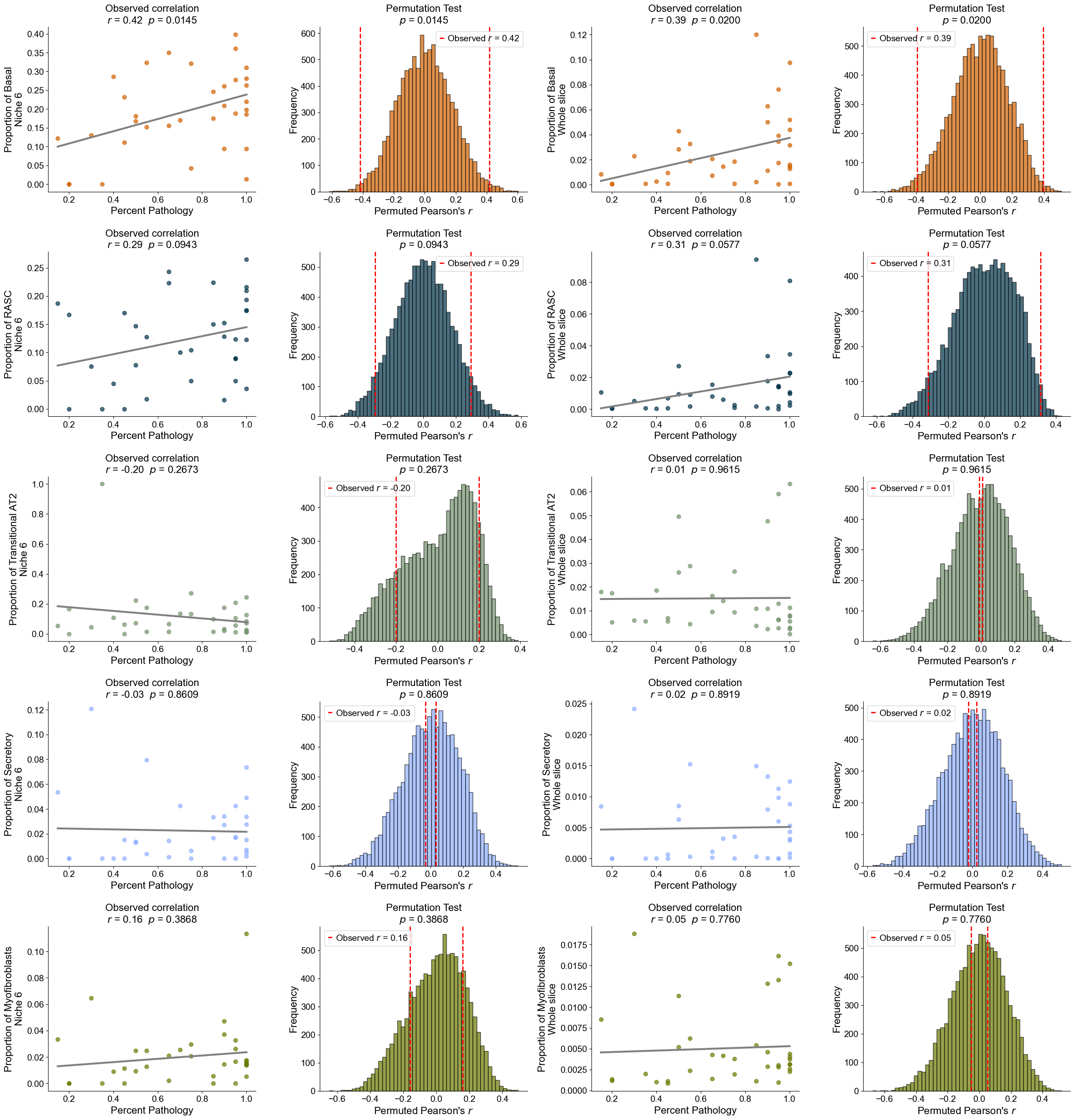
Niche 7: Macrophage aggregates
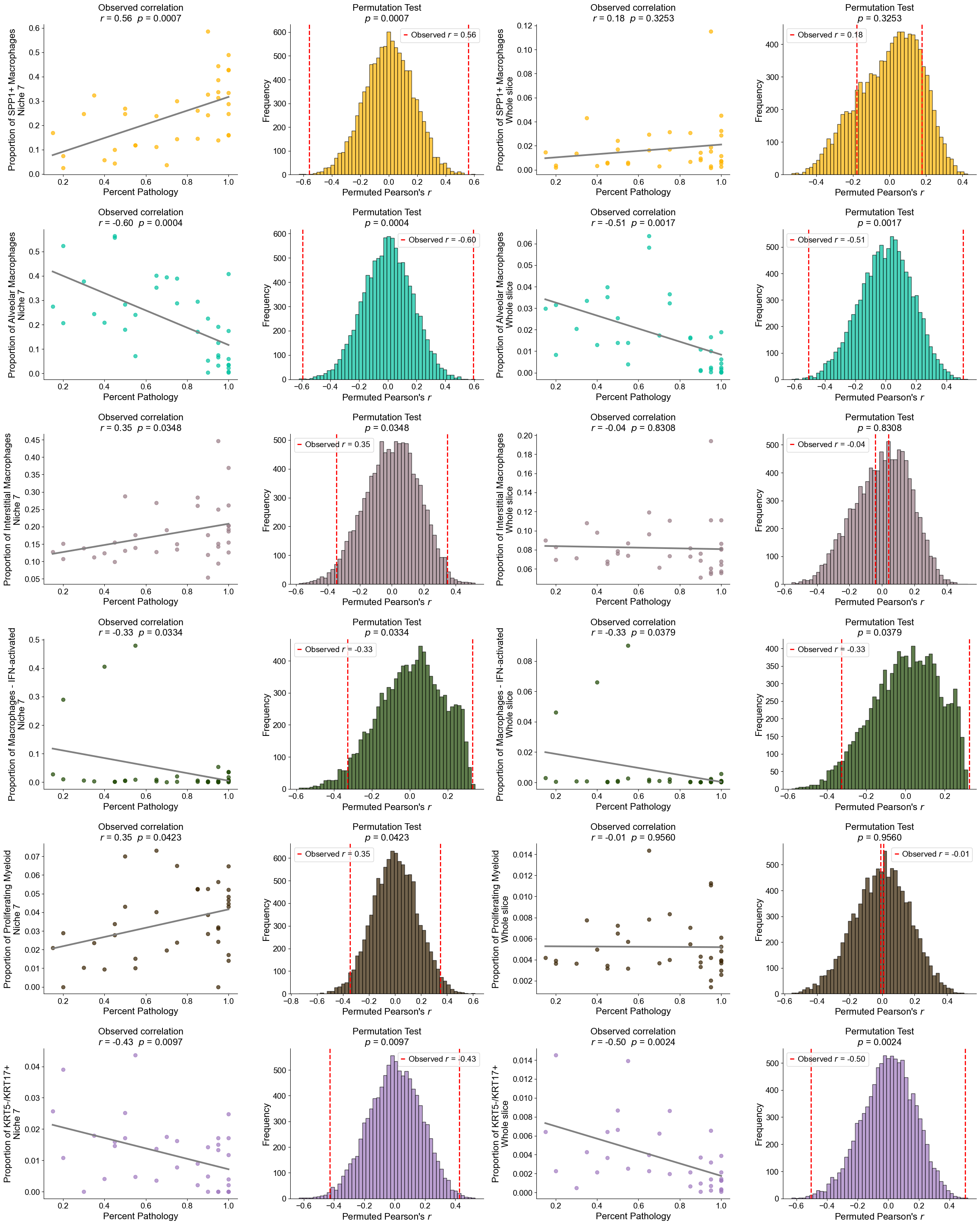
Proportion of SPP1+ macrophages / Proportion of Alveolar macrophages
Perform a Spearman correlation analysis between the log ratio of SPP1+ macrophages to Alveolar macrophages and the percent pathology.
Compute the correlation separately within niche 7 and across the whole slice, and use a permutation test to assess statistical significance.
[30]:
n_permutations = 10000
np.random.seed(1234)

niche = '7'
fig, axes = plt.subplots(1, 4, figsize=(24, 5))

patho_annot = []
ct_prop = []
for i, slice_name in enumerate(cond_name_list):

    adata = cond_concat_new[(cond_concat_new.obs['slice_name'] == slice_name) & (cond_concat_new.obs['niche_label'] == niche), :].copy()
    if adata.shape[0] == 0 or np.mean(adata.obs['final_CT'] == 'Alveolar Macrophages') == 0:
        continue

    patho_annot.append(adata.obs['percent_pathology'][0])
    ct_prop.append(np.log(np.mean(adata.obs['final_CT'] == 'SPP1+ Macrophages') / np.mean(adata.obs['final_CT'] == 'Alveolar Macrophages')))

patho_annot = np.array(patho_annot) / 100
ct_prop  = np.array(ct_prop)

obs_r, _ = spearmanr(patho_annot, ct_prop)

perm_rs = np.zeros(n_permutations)
for i in range(n_permutations):
    permuted = np.random.permutation(ct_prop)
    perm_rs[i], _ = spearmanr(patho_annot, permuted)

p_perm = np.mean(np.abs(perm_rs) >= np.abs(obs_r))

axes[0].scatter(patho_annot, ct_prop, color='springgreen', s=40, alpha=0.7)
m, b = np.polyfit(patho_annot, ct_prop, 1)
x_line = np.linspace(min(patho_annot), max(patho_annot), 100)
y_line = m * x_line + b
axes[0].plot(x_line, y_line,  color='gray', linewidth=3)
axes[0].set_title(f'Observed correlation\n$\\rho$ = {obs_r:.2f}  $p$ = {p_perm:.4f}', fontsize=16)
axes[0].set_xlabel('Percent Pathology', fontsize=16)
axes[0].set_ylabel(f'SPP1+ Macrophages / Alveolar Macrophages\nNiche {niche}', fontsize=16)
axes[0].spines['top'].set_visible(False)
axes[0].spines['right'].set_visible(False)
axes[0].grid(False)

axes[1].hist(perm_rs, bins=50, color='springgreen', edgecolor='black', alpha=0.7)
axes[1].axvline(obs_r, linestyle='--', color='red', linewidth=2, label=f'Observed $\\rho$ = {obs_r:.2f}')
axes[1].axvline(-obs_r, linestyle='--', color='red', linewidth=2)
axes[1].set_title(f'Permutation Test\n$p$ = {p_perm:.4f}', fontsize=16)
axes[1].set_xlabel("Permuted Spearman's $\\rho$", fontsize=16)
axes[1].set_ylabel('Frequency', fontsize=16)
axes[1].spines['top'].set_visible(False)
axes[1].spines['right'].set_visible(False)
axes[1].grid(False)
axes[1].legend(fontsize=14)

patho_annot = []
ct_prop = []
for i, slice_name in enumerate(cond_name_list):

    adata = cond_concat_new[(cond_concat_new.obs['slice_name'] == slice_name), :].copy()
    if adata.shape[0] == 0 or np.mean(adata.obs['final_CT'] == 'Alveolar Macrophages') == 0:
        continue

    patho_annot.append(adata.obs['percent_pathology'][0])
    ct_prop.append(np.log(np.mean(adata.obs['final_CT'] == 'SPP1+ Macrophages') / np.mean(adata.obs['final_CT'] == 'Alveolar Macrophages')))

patho_annot = np.array(patho_annot) / 100
ct_prop  = np.array(ct_prop)

obs_r, _ = spearmanr(patho_annot, ct_prop)

perm_rs = np.zeros(n_permutations)
for i in range(n_permutations):
    permuted = np.random.permutation(ct_prop)
    perm_rs[i], _ = spearmanr(patho_annot, permuted)

p_perm = np.mean(np.abs(perm_rs) >= np.abs(obs_r))

axes[2].scatter(patho_annot, ct_prop, color='springgreen', s=40, alpha=0.7)
m, b = np.polyfit(patho_annot, ct_prop, 1)
x_line = np.linspace(min(patho_annot), max(patho_annot), 100)
y_line = m * x_line + b
axes[2].plot(x_line, y_line,  color='gray', linewidth=3)
axes[2].set_title(f'Observed correlation\n$\\rho$ = {obs_r:.2f}  $p$ = {p_perm:.4f}', fontsize=16)
axes[2].set_xlabel('Percent Pathology', fontsize=16)
axes[2].set_ylabel(f'SPP1+ Macrophages / Alveolar Macrophages\nWhole slice', fontsize=16)
axes[2].spines['top'].set_visible(False)
axes[2].spines['right'].set_visible(False)
axes[2].grid(False)

axes[3].hist(perm_rs, bins=50, color='springgreen', edgecolor='black', alpha=0.7)
axes[3].axvline(obs_r, linestyle='--', color='red', linewidth=2, label=f'Observed $\\rho$ = {obs_r:.2f}')
axes[3].axvline(-obs_r, linestyle='--', color='red', linewidth=2)
axes[3].set_title(f'Permutation Test\n$p$ = {p_perm:.4f}', fontsize=16)
axes[3].set_xlabel("Permuted Spearman's $\\rho$", fontsize=16)
axes[3].set_ylabel('Frequency', fontsize=16)
axes[3].spines['top'].set_visible(False)
axes[3].spines['right'].set_visible(False)
axes[3].grid(False)
axes[3].legend(fontsize=14)

plt.tight_layout()
plt.show()
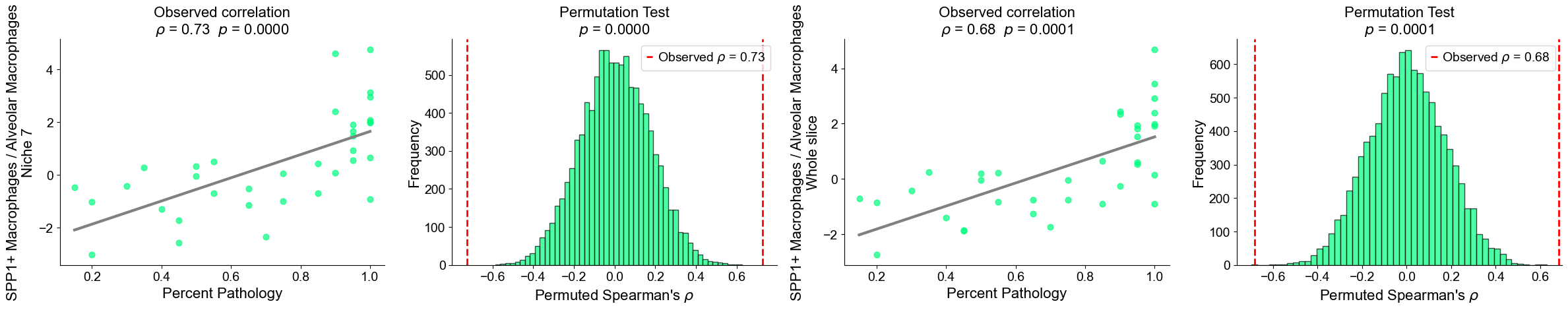
Niche-niche co-localization analysis
control group
[31]:
nnc_results = nnc_enrichment_test(ctr_list,
                                  'niche_label',
                                  niche_summary=ctr_concat_new.uns['niche_label_summary'],
                                  spatial_key='spatial',
                                  cut_percentage=99,
                                  method='fisher',
                                  alpha=0.05,
                                  fdr_method='fdr_by',
                                  log2fc_threshold=1,
                                  prop_threshold=0.01,
                                  verbose=True,
                                  )
nnc_df, edge_prop_mtx, n1_count = nnc_results
nnc_df.head()
4 niches in total.
[31]:
| niche1_idx | niche1 | niche2_idx | niche2 | edge_count | edge_prop | oddsratio | p-value | q-value | log2fc | enrichment | |
|---|---|---|---|---|---|---|---|---|---|---|---|
| 0 | 0 | 0 | 1 | 1 | 272.0 | 0.007031 | 0.221407 | 4.986353e-160 | 3.094741e-159 | -2.139988 | False |
| 1 | 0 | 0 | 2 | 2 | 7131.0 | 0.184330 | 1.432723 | 5.214841e-88 | 2.427412e-87 | 0.436118 | False |
| 2 | 0 | 0 | 3 | 3 | 31283.0 | 0.808639 | 27.089002 | 0.000000e+00 | 0.000000e+00 | 2.583139 | True |
| 3 | 1 | 1 | 0 | 0 | 272.0 | 0.136683 | 0.221407 | 4.986353e-160 | 3.094741e-159 | -1.608988 | False |
| 4 | 1 | 1 | 2 | 2 | 895.0 | 0.449749 | 4.643949 | 1.171986e-216 | 1.091076e-215 | 1.587407 | True |
[34]:
niche_labels = ctr_concat_new.uns['niche_label_summary'].copy()

nnc_df['stars'] = nnc_df['q-value'].apply(p2stars)

matrix_df = pd.DataFrame(
    data=edge_prop_mtx,
    index=niche_labels,
    columns=niche_labels,
)

for i in range(matrix_df.shape[0]):
    for j in range(matrix_df.shape[1]):
        if i == j:
            matrix_df.iloc[i, j] = np.nan

stars_df = pd.DataFrame(
    '',
    index=matrix_df.index,
    columns=matrix_df.columns
)

for _, row in nnc_df[nnc_df['enrichment']].iterrows():
    n1 = row['niche1']
    n2 = row['niche2']
    if (n1 in stars_df.index) and (n2 in stars_df.columns):
        stars_df.loc[n1, n2] = row['stars']

plt.figure(figsize=(4, 3.5))

ax  = sns.heatmap(
    matrix_df,
    cmap='Greens',
    # cbar_kws={'label': 'Edge type proportion'},
    linewidths=0.7,
    linecolor='gray',
    # square=True,
)

for i, n1 in enumerate(matrix_df.index):
    for j, n2 in enumerate(matrix_df.columns):
        if i == j:
            ax.plot([i, i+1], [i, i+1], color='gray', linewidth=0.7)
            # ax.plot([i+1, i], [i, i+1], color='gray', linewidth=0.7)
            continue
        star = stars_df.iloc[i, j]
        if star:
            if matrix_df.iloc[i, j] > np.nanmax(matrix_df.values) * 0.7:
                color='white'
            else:
                color='black'
            ax.text(j + 0.5, i + 0.6, star, ha='center', va='center', color=color, fontsize=20, fontweight='bold')

n_rows, n_cols = matrix_df.shape
ax.plot([0, n_cols], [n_rows, n_rows], color='gray', linewidth=0.7, clip_on=False)
ax.plot([n_cols, n_cols], [0, n_rows], color='gray', linewidth=0.7, clip_on=False)

ax.set_xticklabels(ax.get_xticklabels(), rotation=0, ha='center', fontsize=16)
ax.set_yticklabels(ax.get_yticklabels(), rotation=0, ha='right', fontsize=16)
ax.set_ylabel('Niche', fontsize=16)
ax.set_xlabel('Niche', fontsize=16)
ax.set_title('Edge Type Proportions', fontsize=16)
ax.collections[0].colorbar.ax.yaxis.label.set_size(16)
ax.collections[0].colorbar.ax.tick_params(labelsize=16)
ax.grid(False)

plt.tight_layout()
plt.show()
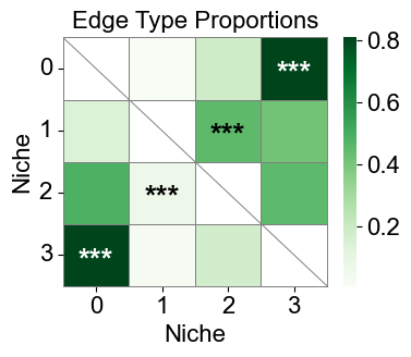
condition group
[35]:
nnc_results = nnc_enrichment_test(cond_list,
                                  'niche_label',
                                  niche_summary=cond_concat_new.uns['niche_label_summary'],
                                  spatial_key='spatial',
                                  cut_percentage=99,
                                  method='fisher',
                                  alpha=0.05,
                                  fdr_method='fdr_by',
                                  log2fc_threshold=1,
                                  prop_threshold=0.01,
                                  verbose=True,
                                  )
nnc_df, edge_prop_mtx, n1_count = nnc_results
nnc_df.head()
8 niches in total.
[35]:
| niche1_idx | niche1 | niche2_idx | niche2 | edge_count | edge_prop | oddsratio | p-value | q-value | log2fc | enrichment | |
|---|---|---|---|---|---|---|---|---|---|---|---|
| 0 | 0 | 0 | 1 | 1 | 662.0 | 0.003088 | 0.087907 | 0.0 | 0.0 | -3.462377 | False |
| 1 | 0 | 0 | 2 | 2 | 15324.0 | 0.071481 | 0.296129 | 0.0 | 0.0 | -1.529313 | False |
| 2 | 0 | 0 | 3 | 3 | 68578.0 | 0.319893 | 2.604165 | 0.0 | 0.0 | 1.064196 | True |
| 3 | 0 | 0 | 4 | 4 | 13493.0 | 0.062940 | 0.341470 | 0.0 | 0.0 | -1.384893 | False |
| 4 | 0 | 0 | 5 | 5 | 87845.0 | 0.409767 | 2.806099 | 0.0 | 0.0 | 1.046854 | True |
[38]:
niche_labels = cond_concat_new.uns['niche_label_summary'].copy()

nnc_df['stars'] = nnc_df['q-value'].apply(p2stars)

matrix_df = pd.DataFrame(
    data=edge_prop_mtx,
    index=niche_labels,
    columns=niche_labels,
)

for i in range(matrix_df.shape[0]):
    for j in range(matrix_df.shape[1]):
        if i == j:
            matrix_df.iloc[i, j] = np.nan

stars_df = pd.DataFrame(
    '',
    index=matrix_df.index,
    columns=matrix_df.columns
)

for _, row in nnc_df[nnc_df['enrichment']].iterrows():
    n1 = row['niche1']
    n2 = row['niche2']
    if (n1 in stars_df.index) and (n2 in stars_df.columns):
        stars_df.loc[n1, n2] = row['stars']

plt.figure(figsize=(5.8, 5))

ax  = sns.heatmap(
    matrix_df,
    cmap='Greens',
    # cbar_kws={'label': 'Edge type proportion'},
    linewidths=0.7,
    linecolor='gray',
    # square=True,
)

for i, n1 in enumerate(matrix_df.index):
    for j, n2 in enumerate(matrix_df.columns):
        if i == j:
            ax.plot([i, i+1], [i, i+1], color='gray', linewidth=0.7)
            # ax.plot([i+1, i], [i, i+1], color='gray', linewidth=0.7)
            continue
        star = stars_df.iloc[i, j]
        if star:
            if matrix_df.iloc[i, j] > np.nanmax(matrix_df.values) * 0.7:
                color='white'
            else:
                color='black'
            ax.text(j + 0.5, i + 0.6, star, ha='center', va='center', color=color, fontsize=20, fontweight='bold')

n_rows, n_cols = matrix_df.shape
ax.plot([0, n_cols], [n_rows, n_rows], color='gray', linewidth=0.7, clip_on=False)
ax.plot([n_cols, n_cols], [0, n_rows], color='gray', linewidth=0.7, clip_on=False)

ax.set_xticklabels(ax.get_xticklabels(), rotation=0, ha='center', fontsize=16)
ax.set_yticklabels(ax.get_yticklabels(), rotation=0, ha='right', fontsize=16)
ax.set_ylabel('Niche', fontsize=16)
ax.set_xlabel('Niche', fontsize=16)
ax.set_title('Edge Type Proportions', fontsize=16)
ax.collections[0].colorbar.ax.yaxis.label.set_size(16)
ax.collections[0].colorbar.ax.tick_params(labelsize=16)
ax.grid(False)

plt.tight_layout()
plt.show()
niche_annot
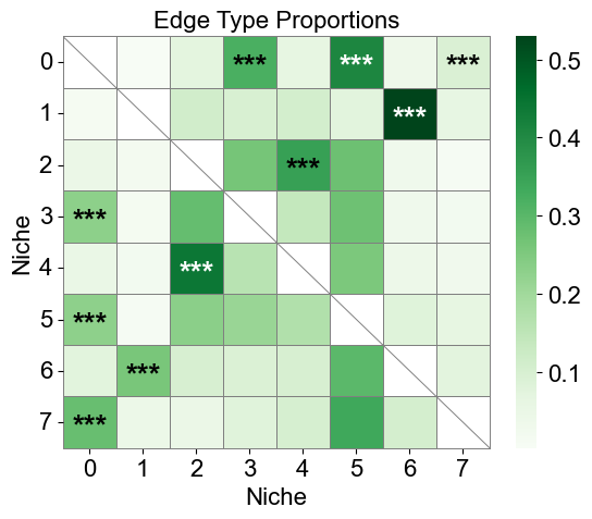
[38]:
{'0': 'Alveolar epithelium',
 '1': 'Airway epithelium',
 '2': 'Interstitial fibrotic',
 '3': 'Vascular',
 '4': 'Lymphoid immune aggregates',
 '5': 'Fibrotic foci',
 '6': 'Aberrant epithelium',
 '7': 'Macrophage aggregates'}
Niche affinity
Calculate how often cells from niche 6 are adjacent to cells from other niches. For each slice, identify all neighboring cell pairs using the Delaunay adjacency matrix. Count how many neighbors from each other niche are next to niche 6 and record the proportion for each slice.
[57]:
source_niche = '6'
min_cell_count = 20

other_niches = [n for n in cond_concat_new.uns['niche_label_summary'] if n != source_niche]
count_dict = {n: [] for n in other_niches}
for i, slice_name in enumerate(cond_name_list):

    if (cond_list[i].obs['niche_label'] == source_niche).sum() < min_cell_count:
        print(f'Skipping {slice_name} due to few cell counts ({(cond_list[i].obs["niche_label"] == source_niche).sum()}).')
        continue

    adj_mtx = cond_list[i].obsp['delaunay_adj_mtx']
    labels = cond_list[i].obs['niche_label']

    rows, cols = adj_mtx.nonzero()

    pairs = [(labels[j1], labels[j2]) for j1, j2 in zip(rows, cols) if ((labels[j1] == source_niche) and (labels[j2] != source_niche))]

    ratio_map = {n: 0.0 for n in other_niches}
    if len(pairs) > 0:
        pair_counts = pd.Series(pairs).value_counts()
        for (n1, n2), count in pair_counts.items():
            ratio_map[n2] = count / len(pairs)
    for n2 in other_niches:
        count_dict[n2].append(ratio_map[n2])
Skipping TILD111LA due to few cell counts (6).
Skipping VUILD102LA due to few cell counts (1).
Skipping VUILD102MA due to few cell counts (0).
Skipping VUILD48LA1 due to few cell counts (13).
Skipping VUILD49LA due to few cell counts (9).
[58]:
np.random.seed(1234)
def add_jitter(x, scale=0.1):
    return x + np.random.normal(0, scale, size=len(x))

prop_list = [count_dict[niche] for niche in cond_concat_new.uns['niche_label_summary'] if niche != source_niche]
palette = [niche_color_dict[niche] for niche in cond_concat_new.uns['niche_label_summary'] if niche != source_niche]
niche_labels = [niche for niche in cond_concat_new.uns['niche_label_summary'] if niche != source_niche]

fig, ax = plt.subplots(1, 1, figsize=(6, 4))
x_pos = np.arange(len(palette))

sns.boxplot(data=prop_list, ax=ax, showfliers=False, palette=palette, width=0.7)
for i, prop in enumerate(prop_list):
    ax.scatter(add_jitter(np.full(len(prop), x_pos[i])), prop, color='white', edgecolor="black", alpha=0.8, s=30, zorder=2)
ax.set_xticks(x_pos)
ax.set_xticklabels(niche_labels, rotation=0, ha='center', fontsize=16)
ax.set_yticklabels(ax.get_yticklabels(), rotation=0, ha='right', fontsize=16)
ax.set_ylabel("Edge Proportion", fontsize=16)
ax.set_title(f"Relative adjacency frequency with niche {source_niche}", fontsize=16)
ax.grid(False)
ax.spines['right'].set_visible(False)
ax.spines['top'].set_visible(False)
plt.tight_layout()
plt.show()
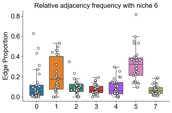
Calculate the proportion of SPP1+ Macrophages within niche 7 for each slice. Record the pathology percentage for each slice. Identify all neighboring cell pairs using the Delaunay adjacency matrix and count how often cells from niche 7 are adjacent to cells from other niches. For each other niche, store the proportion of these neighboring pairs relative to all niche 7 adjacency pairs.
[59]:
source_niche = '7'
min_cell_count = 20

other_niches = [n for n in cond_concat_new.uns['niche_label_summary'] if n != source_niche]
count_dict = {n: [] for n in other_niches}
ctoi_prop = []
patho_annot = []

for i, slice_name in enumerate(cond_name_list):

    if (cond_list[i].obs['niche_label'] == source_niche).sum() < min_cell_count:
        print(f'Skipping {slice_name} due to few cell counts ({(cond_list[i].obs["niche_label"] == source_niche).sum()}).')
        continue

    ctoi_prop.append(((cond_list[i].obs['final_CT'] == 'SPP1+ Macrophages') &
                      (cond_list[i].obs['niche_label'] == source_niche)).sum() /
                      (cond_list[i].obs['niche_label'] == source_niche).sum())
    patho_annot.append(cond_list[i].obs['percent_pathology'][0] / 100)

    adj_mtx = cond_list[i].obsp['delaunay_adj_mtx']
    labels = cond_list[i].obs['niche_label']

    rows, cols = adj_mtx.nonzero()

    pairs = [(labels[j1], labels[j2]) for j1, j2 in zip(rows, cols) if ((labels[j1] == source_niche) and (labels[j2] != source_niche))]

    ratio_map = {n: 0.0 for n in other_niches}
    if len(pairs) > 0:
        pair_counts = pd.Series(pairs).value_counts()
        for (n1, n2), count in pair_counts.items():
            ratio_map[n2] = count / len(pairs)
    for n2 in other_niches:
        count_dict[n2].append(ratio_map[n2])
Skipping VUILD105MA2 due to few cell counts (16).
[60]:
np.random.seed(1234)
def add_jitter(x, scale=0.1):
    return x + np.random.normal(0, scale, size=len(x))

prop_list = [count_dict[niche] for niche in cond_concat_new.uns['niche_label_summary'] if niche != source_niche]
palette = [niche_color_dict[niche] for niche in cond_concat_new.uns['niche_label_summary'] if niche != source_niche]
niche_labels = [niche for niche in cond_concat_new.uns['niche_label_summary'] if niche != source_niche]

fig, ax = plt.subplots(1, 1, figsize=(6, 4))
x_pos = np.arange(len(palette))

sns.boxplot(data=prop_list, ax=ax, showfliers=False, palette=palette, width=0.7)
for i, prop in enumerate(prop_list):
    ax.scatter(add_jitter(np.full(len(prop), x_pos[i])), prop, color='white', edgecolor="black", alpha=0.8, s=30, zorder=2)
ax.set_xticks(x_pos)
ax.set_xticklabels(niche_labels, rotation=0, ha='center', fontsize=16)
ax.set_yticklabels(ax.get_yticklabels(), rotation=0, ha='right', fontsize=16)
ax.set_ylabel("Edge Proportion", fontsize=16)
ax.set_title(f"Relative adjacency frequency with niche {source_niche}", fontsize=16)
ax.grid(False)
ax.spines['right'].set_visible(False)
ax.spines['top'].set_visible(False)
plt.tight_layout()
plt.show()
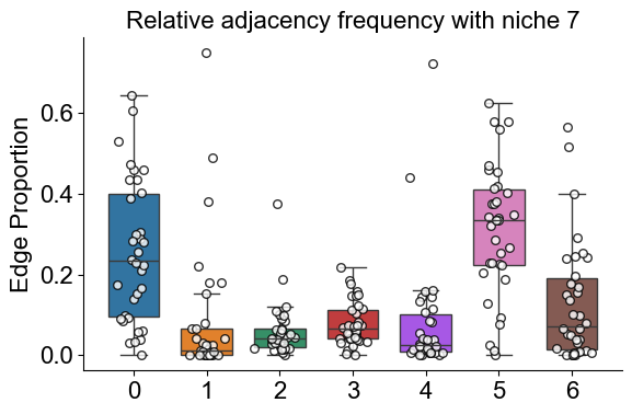
Compare niche 7 edge proportions with pathology percentage and with the proportion of SPP1+ Macrophages in niche 7 across slices. Perform a permutation test to assess significance of observed correlations. Visualize each comparison with a scatter plot and regression line, and show the distribution of correlation coefficients from permutations.
[62]:
n_permutations = 10000
np.random.seed(1234)

patho_annot = np.array(patho_annot)
ctoi_prop  = np.array(ctoi_prop)

for niche in niche_labels:

    edge_prop = np.array(count_dict[niche])

    fig, axes = plt.subplots(1, 4, figsize=(24, 5))

    obs_r, _ = pearsonr(patho_annot, edge_prop)

    perm_rs = np.zeros(n_permutations)
    for i in range(n_permutations):
        permuted = np.random.permutation(edge_prop)
        perm_rs[i], _ = pearsonr(patho_annot, permuted)

    p_perm = np.mean(np.abs(perm_rs) >= np.abs(obs_r))

    axes[0].scatter(patho_annot, edge_prop, color=niche_color_dict[niche], s=40, alpha=0.7)
    m, b = np.polyfit(patho_annot, edge_prop, 1)
    x_line = np.linspace(min(patho_annot), max(patho_annot), 100)
    y_line = m * x_line + b
    axes[0].plot(x_line, y_line,  color='gray', linewidth=3)
    axes[0].set_title(f'Observed correlation\n$r$ = {obs_r:.2f}  $p$ = {p_perm:.4f}', fontsize=16)
    axes[0].set_xlabel('Percent Pathology', fontsize=16)
    axes[0].set_ylabel(f'Niche {niche} Edge Proportion', fontsize=16)
    axes[0].spines['top'].set_visible(False)
    axes[0].spines['right'].set_visible(False)
    axes[0].grid(False)

    axes[1].hist(perm_rs, bins=50, color=niche_color_dict[niche], edgecolor='black', alpha=0.7)
    axes[1].axvline(obs_r, linestyle='--', color='red', linewidth=2, label=f'Observed $r$ = {obs_r:.2f}')
    axes[1].axvline(-obs_r, linestyle='--', color='red', linewidth=2)
    axes[1].set_title(f'Permutation Test\n$p$ = {p_perm:.4f}', fontsize=16)
    axes[1].set_xlabel("Permuted Pearson's $r$", fontsize=16)
    axes[1].set_ylabel('Frequency', fontsize=16)
    axes[1].spines['top'].set_visible(False)
    axes[1].spines['right'].set_visible(False)
    axes[1].grid(False)
    axes[1].legend(fontsize=14)

    obs_r, _ = pearsonr(ctoi_prop, edge_prop)

    perm_rs = np.zeros(n_permutations)
    for i in range(n_permutations):
        permuted = np.random.permutation(edge_prop)
        perm_rs[i], _ = pearsonr(ctoi_prop, permuted)

    p_perm = np.mean(np.abs(perm_rs) >= np.abs(obs_r))

    axes[2].scatter(ctoi_prop, edge_prop, color=niche_color_dict[niche], s=40, alpha=0.7)
    m, b = np.polyfit(ctoi_prop, edge_prop, 1)
    x_line = np.linspace(min(ctoi_prop), max(ctoi_prop), 100)
    y_line = m * x_line + b
    axes[2].plot(x_line, y_line,  color='gray', linewidth=3)
    axes[2].set_title(f'Observed correlation\n$r$ = {obs_r:.2f}  $p$ = {p_perm:.4f}', fontsize=16)
    axes[2].set_xlabel(f'SPP1+ Macrophages Proportion Niche {source_niche}', fontsize=16)
    axes[2].set_ylabel(f'Niche {niche} Edge Proportion', fontsize=16)
    axes[2].spines['top'].set_visible(False)
    axes[2].spines['right'].set_visible(False)
    axes[2].grid(False)

    axes[3].hist(perm_rs, bins=50, color=niche_color_dict[niche], edgecolor='black', alpha=0.7)
    axes[3].axvline(obs_r, linestyle='--', color='red', linewidth=2, label=f'Observed $r$ = {obs_r:.2f}')
    axes[3].axvline(-obs_r, linestyle='--', color='red', linewidth=2)
    axes[3].set_title(f'Permutation Test\n$p$ = {p_perm:.4f}', fontsize=16)
    axes[3].set_xlabel("Permuted Pearson's $r$", fontsize=16)
    axes[3].set_ylabel('Frequency', fontsize=16)
    axes[3].spines['top'].set_visible(False)
    axes[3].spines['right'].set_visible(False)
    axes[3].grid(False)
    axes[3].legend(fontsize=14)

    plt.tight_layout()
    plt.show()
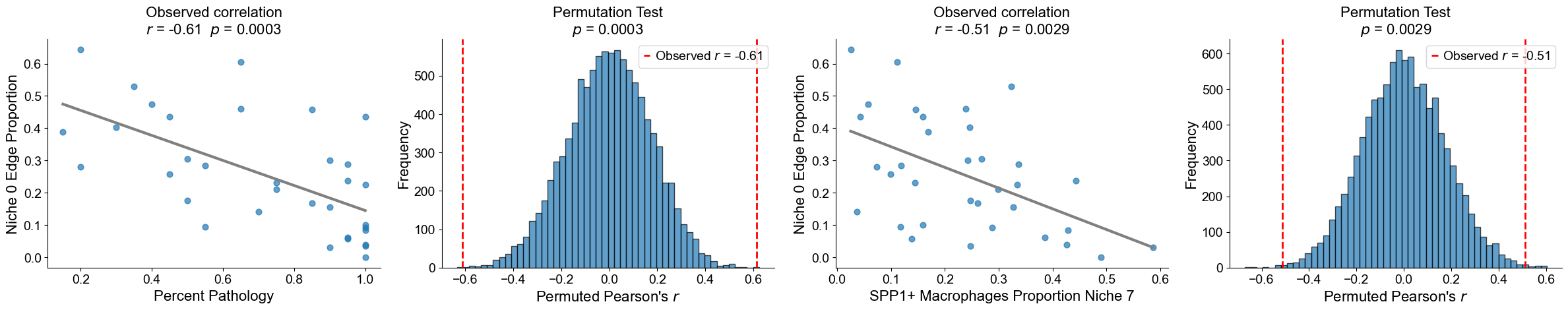
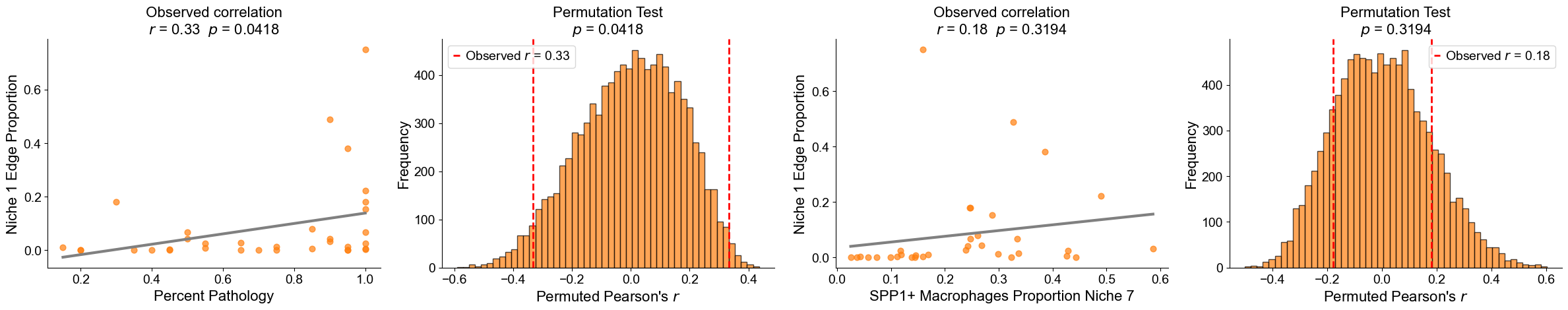
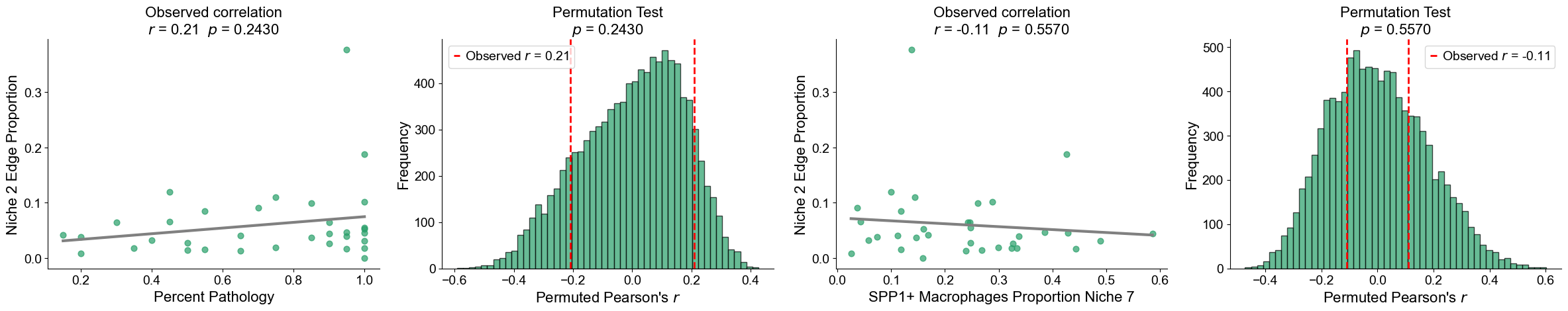
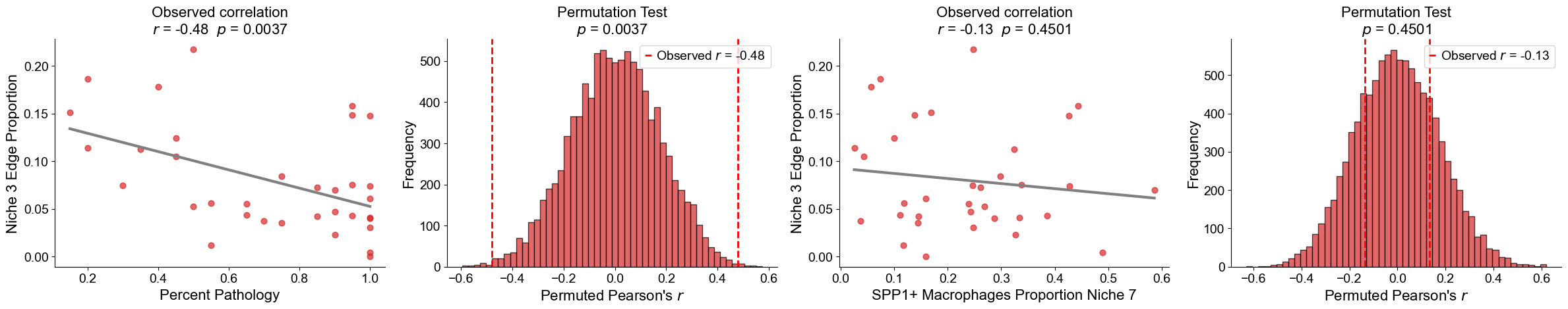
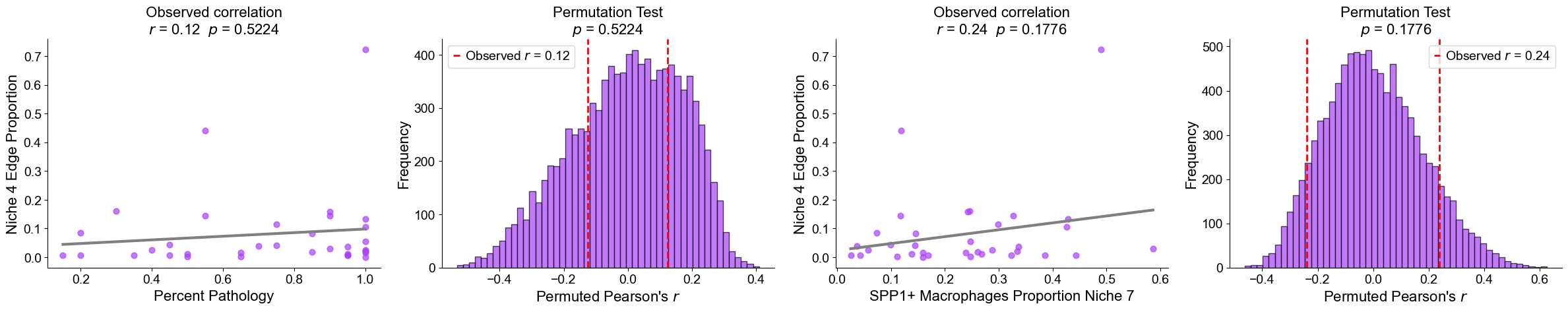
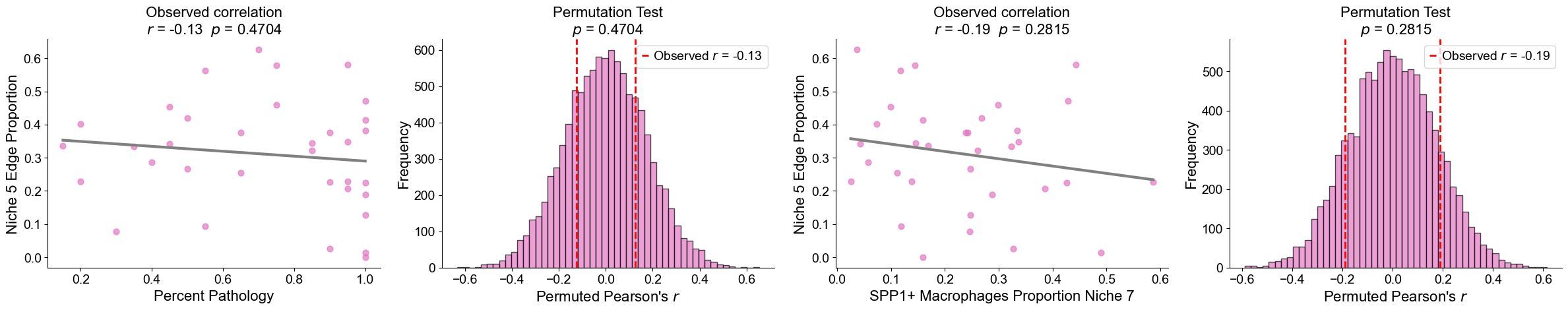
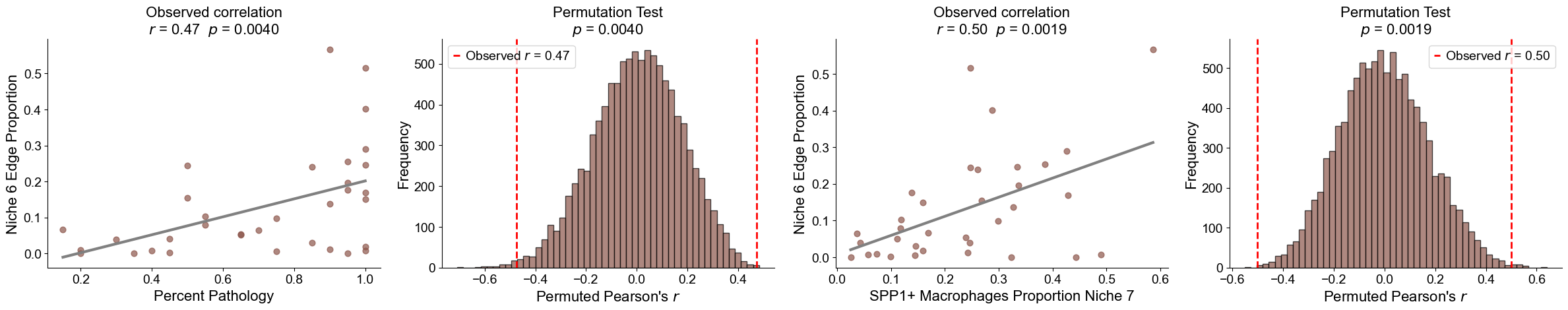
Differentiation (AT2)
Mapping niche 6 to niche 0 & 1
Map niche 6 cells onto niches 0 and 1 using PCA projection, concatenate datasets, and compute neighbors and UMAP.
[8]:
ctoi_list = ['AT2', 'Transitional AT2', 'Basal', 'RASC']

ref = (cond_concat_new.obs['final_CT'].isin(ctoi_list)) & (cond_concat_new.obs['niche_label'].isin(['0', '1'])) & (cond_concat_new.obs['slice_name'] != 'VUILD110LA')
query = (cond_concat_new.obs['final_CT'].isin(ctoi_list)) & (cond_concat_new.obs['niche_label'].isin(['6'])) & (cond_concat_new.obs['slice_name'] != 'VUILD110LA')
adata_selected = cond_concat_new[ref | query, :].copy()  # a slice with apparent batch effect is removed
print(adata_selected.shape)
sc.pp.filter_cells(adata_selected, min_counts=30)
sc.pp.normalize_total(adata_selected, target_sum=1e4)
sc.pp.log1p(adata_selected)
print(adata_selected.shape)

adata_ref = adata_selected[(adata_selected.obs['niche_label'].isin(['0', '1'])), :].copy()
adata_oi = adata_selected[(adata_selected.obs['niche_label'].isin(['6'])), :].copy()

sc.tl.pca(adata_ref, n_comps=10, random_state=1234)

pcs = adata_ref.varm['PCs']
adata_oi.obsm['X_pca'] = (adata_oi.X - adata_ref.X.mean(axis=0)) @ pcs

adata_selected = ad.concat([adata_ref, adata_oi], label='type', keys=['reference', 'query'])

adata_selected.varm['PCs'] = pcs

sc.pp.neighbors(adata_selected, n_neighbors=15, n_pcs=10, random_state=1234)
sc.tl.umap(adata_selected, random_state=1234)#, min_dist=0.3)
(95497, 343)
(86870, 343)
[9]:
size = 15
ct_query_dict = ct_color_dict.copy()
ct_query_dict['reference'] = 'lightgray'

fig, axes = plt.subplots(1, 3, figsize=(24, 6))
axes = axes.flatten()

sc.pl.umap(adata_selected, color="final_CT", size=size, frameon=False, palette=ct_color_dict,
           alpha=0.7, show=False, ax=axes[0])
axes[0].set_title('Cell Type', fontsize=16)

sc.pl.umap(adata_selected, color="niche_label", size=size, frameon=False, palette=niche_color_dict,
           alpha=0.7, show=False, ax=axes[1])
axes[1].set_title('Niche', fontsize=16)

sc.pl.umap(adata_selected, color="type", size=size, frameon=False, palette={'reference': 'lightgray', 'query': 'red'},
           alpha=0.7, show=False, ax=axes[2])
axes[2].set_title('Data Mapping', fontsize=16)

for j in range(len(axes)):
    axes[j].axis('off')
plt.tight_layout()
plt.show()


fig, axes = plt.subplots(1, 3, figsize=(24, 6))
axes = axes.flatten()

print('Reference')
adata_ref = adata_selected[~(adata_selected.obs['niche_label'].isin(['6'])), :].copy()
sc.pl.umap(adata_ref, color="final_CT", size=size, frameon=False, palette=ct_color_dict,
           alpha=0.7, show=False, ax=axes[0])
axes[0].set_title('Cell Type', fontsize=16)

sc.pl.umap(adata_ref, color="niche_label", size=size, frameon=False, palette=niche_color_dict,
           alpha=0.7, show=False, ax=axes[1])
axes[1].set_title('Niche', fontsize=16)

adata_selected.obs['ct_query'] = [adata_selected.obs['final_CT'][i] if adata_selected.obs['niche_label'][i] == '6' else 'reference' for i in range(adata_selected.shape[0])]
sc.pl.umap(adata_selected, color="ct_query", size=size, frameon=False, palette=ct_query_dict,
           alpha=0.7, show=False, ax=axes[2])
axes[2].set_title('Data Mapping to Reference', fontsize=16)

for j in range(len(axes)):
    axes[j].axis('off')
plt.tight_layout()
plt.show()


fig, axes = plt.subplots(2, 3, figsize=(24, 12))
axes = axes.flatten()

print('Query colored')
adata_selected.obs['ct_query1'] = [adata_selected.obs['final_CT'][i] if adata_selected.obs['niche_label'][i] == '6' and (adata_selected.obs['final_CT'][i] in ['AT2', 'Transitional AT2']) else 'reference' for i in range(adata_selected.shape[0])]
tmp = adata_selected[(adata_selected.obs['niche_label'] != '6') | (adata_selected.obs['ct_query1'] != 'reference'), :].copy()
sc.pl.umap(tmp, color="ct_query1", size=size, frameon=False, palette=ct_query_dict,
           alpha=0.7, show=False, ax=axes[0])
axes[0].set_title('Cell Type', fontsize=16)

adata_selected.obs['ct_query2'] = ['Basal' if adata_selected.obs['niche_label'][i] == '6' and adata_selected.obs['final_CT'][i] == 'Basal' else 'reference' for i in range(adata_selected.shape[0])]
tmp = adata_selected[(adata_selected.obs['niche_label'] != '6') | (adata_selected.obs['ct_query2'] != 'reference'), :].copy()
sc.pl.umap(tmp, color="ct_query2", size=size, frameon=False, palette=ct_query_dict,
           alpha=0.7, show=False, ax=axes[1])
axes[1].set_title('Cell Type', fontsize=16)

adata_selected.obs['ct_query3'] = ['RASC' if adata_selected.obs['niche_label'][i] == '6' and adata_selected.obs['final_CT'][i] == 'RASC' else 'reference' for i in range(adata_selected.shape[0])]
tmp = adata_selected[(adata_selected.obs['niche_label'] != '6') | (adata_selected.obs['ct_query3'] != 'reference'), :].copy()
sc.pl.umap(tmp, color="ct_query3", size=size, frameon=False, palette=ct_query_dict,
           alpha=0.7, show=False, ax=axes[2])
axes[2].set_title('Cell Type', fontsize=16)

adata_selected.obs['ct_query4'] = ['AT2' if adata_selected.obs['niche_label'][i] == '6' and adata_selected.obs['final_CT'][i] == 'AT2' else 'reference' for i in range(adata_selected.shape[0])]
tmp = adata_selected[(adata_selected.obs['niche_label'] != '6') | (adata_selected.obs['ct_query4'] != 'reference'), :].copy()
sc.pl.umap(tmp, color="ct_query4", size=size, frameon=False, palette=ct_query_dict,
           alpha=0.7, show=False, ax=axes[3])
axes[3].set_title('Cell Type', fontsize=16)

adata_selected.obs['ct_query5'] = ['Transitional AT2' if adata_selected.obs['niche_label'][i] == '6' and adata_selected.obs['final_CT'][i] == 'Transitional AT2' else 'reference' for i in range(adata_selected.shape[0])]
tmp = adata_selected[(adata_selected.obs['niche_label'] != '6') | (adata_selected.obs['ct_query5'] != 'reference'), :].copy()
sc.pl.umap(tmp, color="ct_query5", size=size, frameon=False, palette=ct_query_dict,
           alpha=0.7, show=False, ax=axes[4])
axes[4].set_title('Cell Type', fontsize=16)

axes[5].axis('off')

for j in range(len(axes)):
    axes[j].axis('off')
plt.tight_layout()
plt.show()
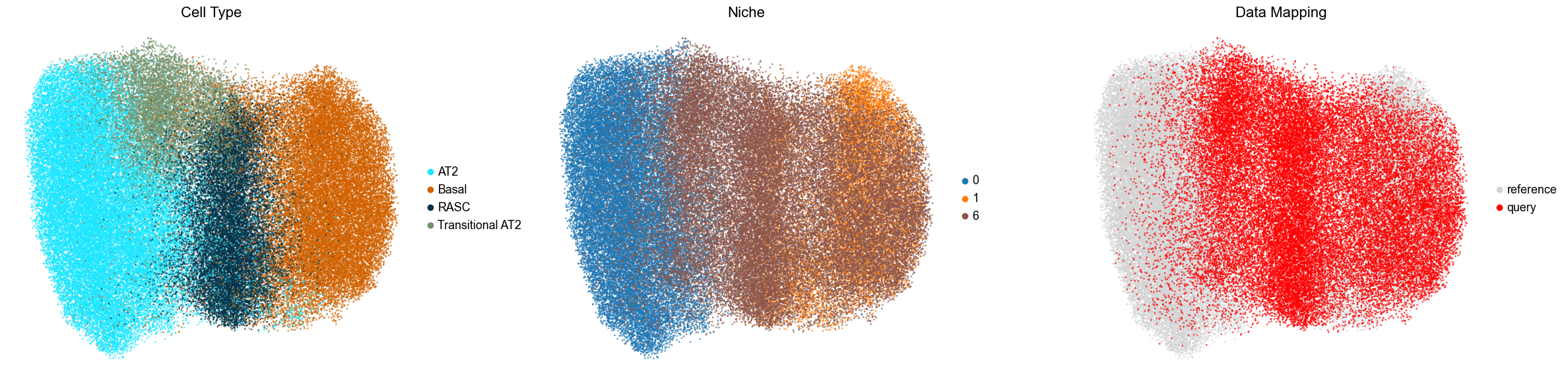
Reference
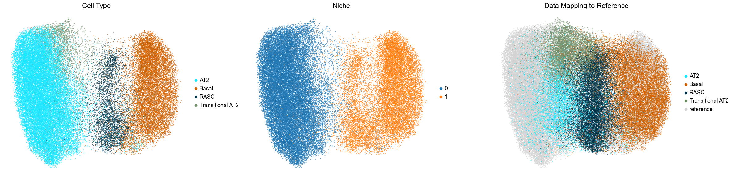
Query colored
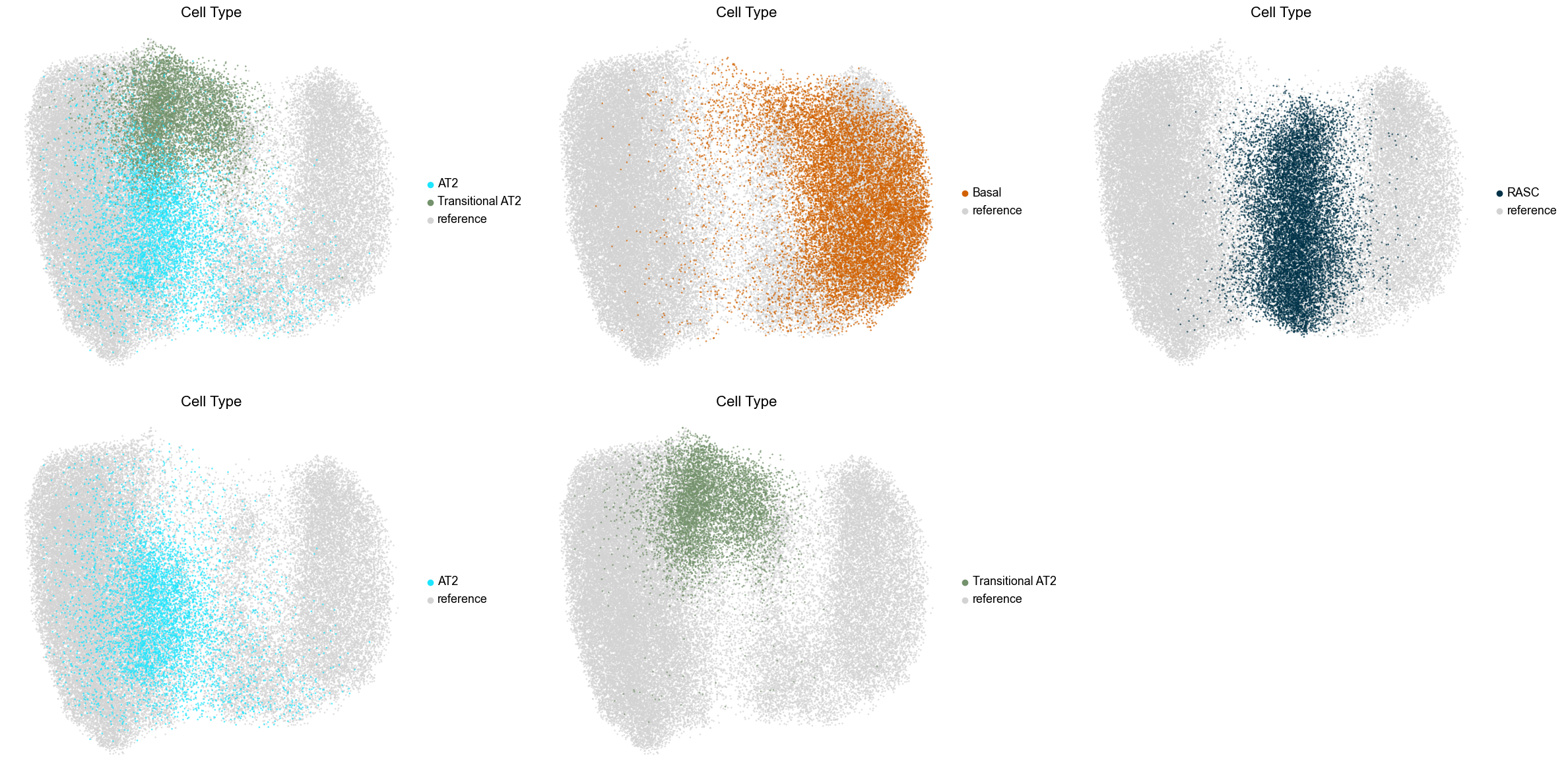
Plot markers
[10]:
size = 10

fig, axes = plt.subplots(2, 4, figsize=(22, 10))
axes = axes.flatten()

genes = ['SFTPC', 'NAPSA', 'LAMP3', 'SCGB3A2', 'SCGB1A1', 'KRT8', 'KRT5', 'KRT17']

for gene, ax in zip(genes, axes):

    sc.pl.umap(adata_selected, color=gene, size=size, frameon=False, palette='viridis',
            alpha=0.7, show=False, ax=ax)
    ax.set_title(gene, fontsize=16)

for j in range(len(axes)):
    axes[j].axis('off')

plt.tight_layout()
plt.show()
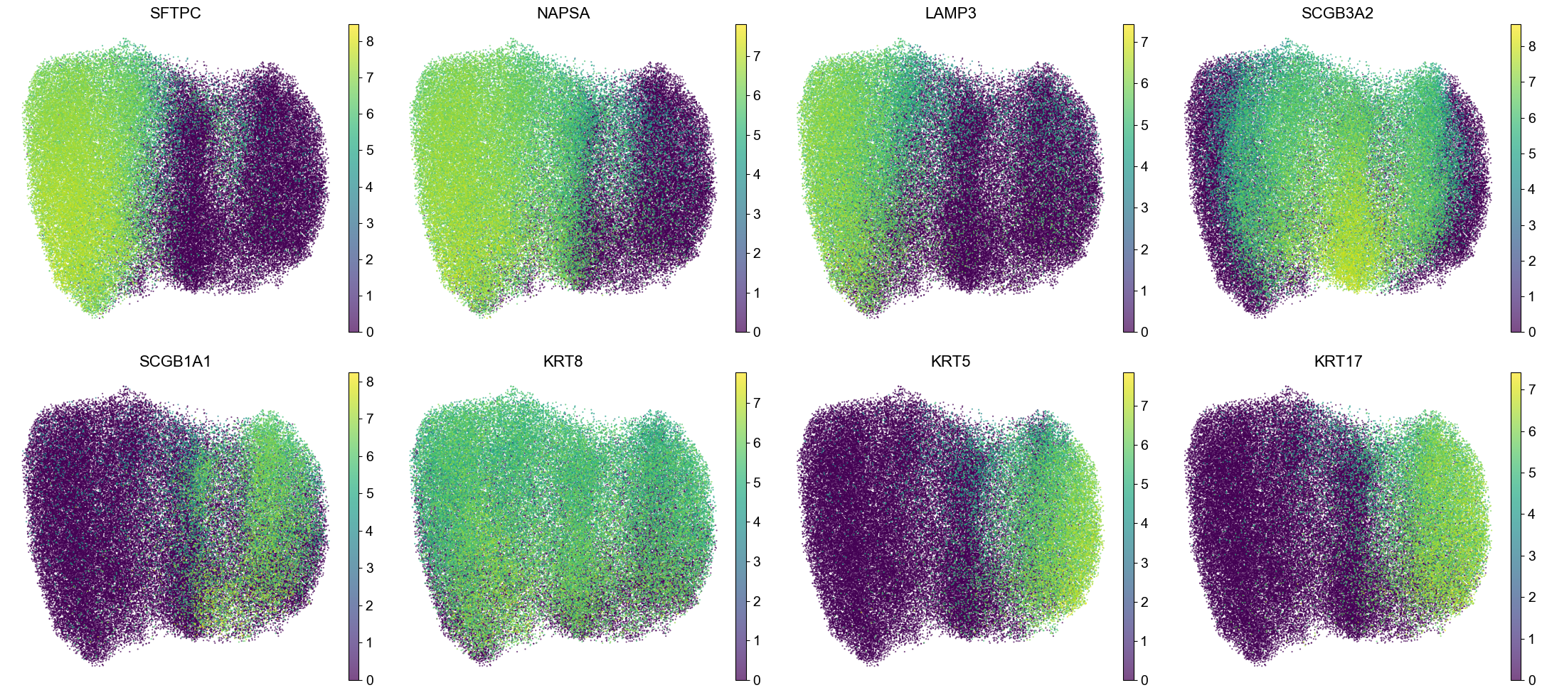
Trajectory inference
Perform trajectory inference using the umap coordinates of the query data
[11]:
from pyslingshot import Slingshot

# ctoi_list = ['AT2', 'Basal', 'RASC', 'Transitional AT2']

# # ref = (cond_concat_new.obs['final_CT'].isin(ctoi_list)) & (cond_concat_new.obs['niche_label'].isin(['0', '1'])) & (cond_concat_new.obs['slice_name'] != 'VUILD110LA')
# # query = (cond_concat_new.obs['final_CT'].isin(ctoi_list)) & (cond_concat_new.obs['niche_label'].isin(['6'])) & (cond_concat_new.obs['slice_name'] != 'VUILD110LA')
# adata_query = cond_concat_new[(cond_concat_new.obs['final_CT'].isin(ctoi_list)) &
#                                  (cond_concat_new.obs['niche_label'].isin(['6'])) &
#                                  (cond_concat_new.obs['slice_name'] != 'VUILD110LA'), :].copy()  # a slice with apparent batch effect is removed

# print(adata_query.shape)
# sc.pp.filter_cells(adata_query, min_counts=30)
# sc.pp.normalize_total(adata_query, target_sum=1e4)
# sc.pp.log1p(adata_query)
# print(adata_query.shape)

# sc.tl.pca(adata_query, n_comps=10, random_state=1234)
# sc.pp.neighbors(adata_query, n_neighbors=5, n_pcs=10, random_state=1234)
# sc.tl.umap(adata_query, random_state=1234)

adata_ref = adata_selected[~(adata_selected.obs['niche_label'].isin(['6'])), :].copy()
adata_query = adata_selected[(adata_selected.obs['niche_label'].isin(['6'])), :].copy()
adata_query
[11]:
AnnData object with n_obs × n_vars = 39379 × 343
    obs: 'sample', 'patient', 'cell_id', 'full_cell_id', 'sample_type', 'sample_affect', 'disease_status', 'percent_pathology', 'tma', 'run', 'final_CT', 'final_lineage', 'CNiche', 'TNiche', 'lumen_id', 'lumen_rank', 'x_centroid', 'y_centroid', 'adj_x_centroid', 'adj_y_centroid', 'super_adj_x_centroid', 'super_adj_y_centroid', 'nCount_RNA', 'nFeature_RNA', 'perc_negcontrolprobe', 'perc_negcontrolcodeword', 'perc_unassigned', 'perc_negcontrolorunassigned', 'slice_name', 'celltype_idx', 'n_neighbors', 'niche_label_10', 'csn_label_10', 'niche_label_9', 'csn_label_9', 'niche_label_8', 'csn_label_8', 'niche_label_7', 'csn_label_7', 'niche_label_6', 'csn_label_6', 'niche_label_5', 'csn_label_5', 'niche_label_4', 'csn_label_4', 'niche_label_3', 'csn_label_3', 'niche_label_2', 'csn_label_2', 'niche_label_1', 'csn_label_1', 'niche_label_0', 'csn_label_0', 'niche_label_jsd_v2', 'csn_label_jsd_v2', 'niche_label_jsd', 'csn_label_jsd', 'niche_label_fmi', 'csn_label_fmi', 'niche_label_ari', 'csn_label_ari', 'niche_label_nmi', 'csn_label_nmi', 'niche_label_asw', 'csn_label_asw', 'niche_label_js_asw', 'csn_label_js_asw', 'niche_label_fisher', 'csn_label_fisher', 'niche_label_chi', 'csn_label_chi', 'niche_label_dbi', 'csn_label_dbi', 'niche_label_dass_mean', 'csn_label_dass_mean', 'niche_label_dass_min', 'csn_label_dass_min', 'niche_label_dafisher', 'csn_label_dafisher', 'niche_label_dachi', 'csn_label_dachi', 'niche_label_0.09', 'csn_label_0.09', 'niche_label_0.11', 'csn_label_0.11', 'niche_label', 'csn_label', 'n_counts', 'type', 'ct_query', 'ct_query1', 'ct_query2', 'ct_query3', 'ct_query4', 'ct_query5'
    uns: 'neighbors', 'umap', 'final_CT_colors', 'niche_label_colors', 'type_colors', 'ct_query_colors'
    obsm: 'micro_dist', 'onehot', 'spatial', 'X_pca', 'X_umap'
    varm: 'PCs'
    obsp: 'distances', 'connectivities'
[12]:
# adata_query.obsm['X_umap'] = adata_query.obsm['X_umap'] / 10
[13]:
slingshot = Slingshot(adata_query, celltype_key="final_CT", obsm_key="X_umap", start_node=0, debug_level='verbose')
[14]:
slingshot.fit(num_epochs=1, debug_axes=None)
Lineages: [Lineage[0, 2, 1], Lineage[0, 3]]
0%| | 0/1 [00:00<?, ?it/s]
Reversing from leaf to root
Averaging branch @0 with lineages: [0, 1] [<pcurvepy2.pcurve.PrincipalCurve object at 0x0000022027974C10>, <pcurvepy2.pcurve.PrincipalCurve object at 0x0000021FD1C87C50>]
Shrinking branch @0 with curves: [<pcurvepy2.pcurve.PrincipalCurve object at 0x0000022027974C10>, <pcurvepy2.pcurve.PrincipalCurve object at 0x0000021FD1C87C50>]
100%|██████████| 1/1 [10:02<00:00, 603.00s/it]
[15]:
adata_query.obs['pseudotime'] = slingshot.unified_pseudotime
Visualize the trajectories and psuedotime
[16]:
size = 15
fig, axes = plt.subplots(1, 3, figsize=(24, 6))
axes = axes.flatten()

sc.pl.umap(adata_ref, color="type", size=size, frameon=False, palette={'reference': 'lightgray'},
           alpha=0.7, show=False, ax=axes[0])
sc.pl.umap(adata_query, color="final_CT", size=size, frameon=False, palette=ct_color_dict,
           alpha=0.7, show=False, ax=axes[0])
for root, kids in slingshot._tree.items():
    for child in kids:
        start = [slingshot.cluster_centres[root][0], slingshot.cluster_centres[child][0]]
        end = [slingshot.cluster_centres[root][1], slingshot.cluster_centres[child][1]]
        axes[0].plot(start, end, c='black', linewidth=2)
axes[0].set_title('Cell Type', fontsize=16)

sc.pl.umap(adata_ref, color="type", size=size, frameon=False, palette={'reference': 'lightgray'},
           alpha=0.7, show=False, ax=axes[1], legend_loc=None)
sc.pl.umap(adata_query, color="pseudotime", size=size, frameon=False, palette='viridis',
           alpha=0.7, show=False, ax=axes[1], colorbar_loc=None)
for root, kids in slingshot._tree.items():
    for child in kids:
        start = [slingshot.cluster_centres[root][0], slingshot.cluster_centres[child][0]]
        end = [slingshot.cluster_centres[root][1], slingshot.cluster_centres[child][1]]
        axes[1].plot(start, end, c='black', linewidth=2)
axes[1].set_title('Pseudotime', fontsize=16)

sc.pl.umap(adata_ref, color="type", size=size, frameon=False, palette={'reference': 'lightgray'},
           alpha=0.7, show=False, ax=axes[2], legend_loc=None)
sc.pl.umap(adata_query, color="pseudotime", size=size, frameon=False, palette='viridis',
           alpha=0.7, show=False, ax=axes[2])
axes[2].set_title('Pseudotime', fontsize=16)

for j in range(len(axes)):
    axes[j].axis('off')
plt.tight_layout()
# plt.savefig(result_dir+"trajectory_1.pdf")
plt.show()


fig, axes = plt.subplots(1, 3, figsize=(24, 6))
axes = axes.flatten()

sc.pl.umap(adata_ref, color="type", size=size, frameon=False, palette={'reference': 'white'},
           alpha=0.7, show=False, ax=axes[0])
sc.pl.umap(adata_query, color="final_CT", size=size, frameon=False, palette=ct_color_dict,
           alpha=0.7, show=False, ax=axes[0])
for root, kids in slingshot._tree.items():
    for child in kids:
        start = [slingshot.cluster_centres[root][0], slingshot.cluster_centres[child][0]]
        end = [slingshot.cluster_centres[root][1], slingshot.cluster_centres[child][1]]
        axes[0].plot(start, end, c='black', linewidth=2)
axes[0].set_title('Cell Type', fontsize=16)

sc.pl.umap(adata_ref, color="type", size=size, frameon=False, palette={'reference': 'white'},
           alpha=0.7, show=False, ax=axes[1], legend_loc=None)
sc.pl.umap(adata_query, color="pseudotime", size=size, frameon=False, palette='viridis',
           alpha=0.7, show=False, ax=axes[1], colorbar_loc=None)
for root, kids in slingshot._tree.items():
    for child in kids:
        start = [slingshot.cluster_centres[root][0], slingshot.cluster_centres[child][0]]
        end = [slingshot.cluster_centres[root][1], slingshot.cluster_centres[child][1]]
        axes[1].plot(start, end, c='black', linewidth=2)
axes[1].set_title('Pseudotime', fontsize=16)

sc.pl.umap(adata_ref, color="type", size=size, frameon=False, palette={'reference': 'white'},
           alpha=0.7, show=False, ax=axes[2], legend_loc=None)
sc.pl.umap(adata_query, color="pseudotime", size=size, frameon=False, palette='viridis',
           alpha=0.7, show=False, ax=axes[2])
axes[2].set_title('Pseudotime', fontsize=16)

for j in range(len(axes)):
    axes[j].axis('off')
plt.tight_layout()
# plt.savefig(result_dir+"trajectory_2.pdf")
plt.show()
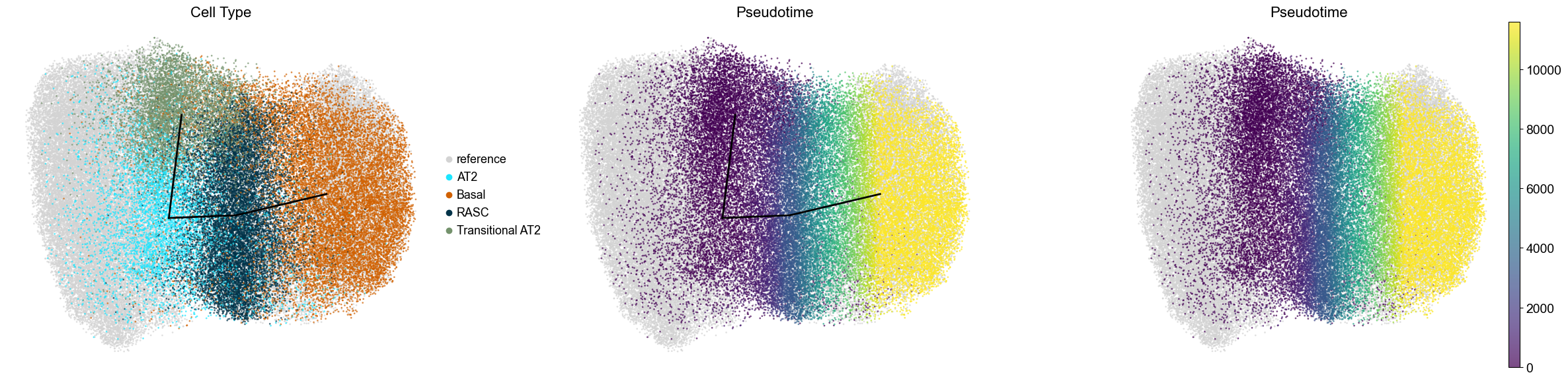
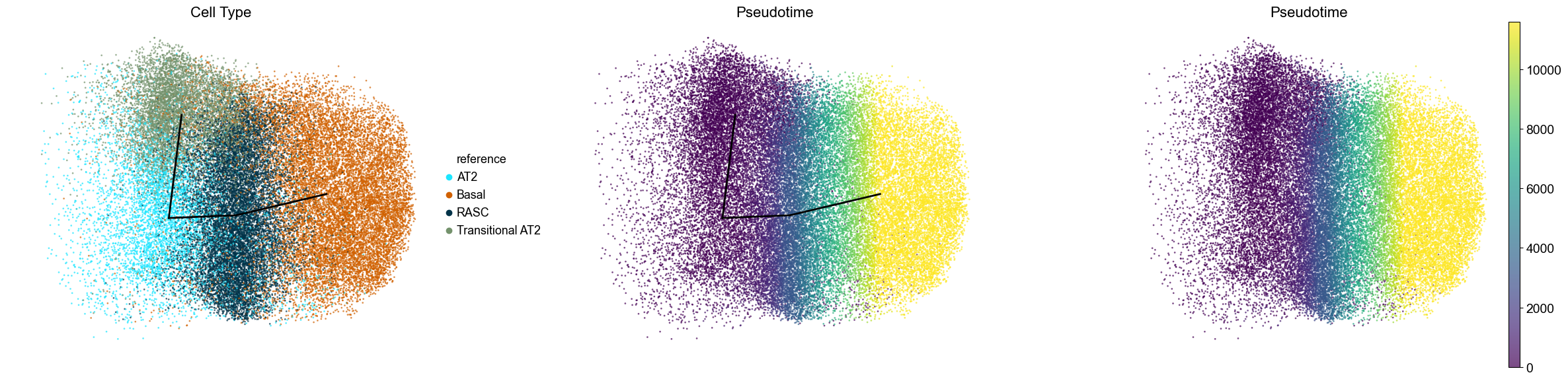
Add AT1 to reference
[75]:
ctoi_list = ['AT2', 'Transitional AT2', 'Basal', 'RASC']
adata_sub = cond_concat_new[(cond_concat_new.obs['slice_name'] != 'VUILD110LA'), :].copy()  # a slice with apparent batch effect is removed
ref = ((adata_sub.obs['final_CT'].isin(ctoi_list)) & (adata_sub.obs['niche_label'].isin(['0', '1']))) | (adata_sub.obs['final_CT'].isin(['AT1']))
query = (adata_sub.obs['final_CT'].isin(ctoi_list)) & (adata_sub.obs['niche_label'].isin(['6']))
adata_selected = adata_sub[ref | query, :].copy()
print(adata_selected.shape)
sc.pp.filter_cells(adata_selected, min_counts=30)
sc.pp.normalize_total(adata_selected, target_sum=1e4)
sc.pp.log1p(adata_selected)
print(adata_selected.shape)

adata_ref = adata_selected[(adata_selected.obs['niche_label'].isin(['0', '1'])) | (adata_selected.obs['final_CT'].isin(['AT1'])), :].copy()
adata_oi = adata_selected[~((adata_selected.obs['niche_label'].isin(['0', '1'])) | (adata_selected.obs['final_CT'].isin(['AT1']))), :].copy()

sc.tl.pca(adata_ref, n_comps=10, random_state=1234)

pcs = adata_ref.varm['PCs']
adata_oi.obsm['X_pca'] = (adata_oi.X - adata_ref.X.mean(axis=0)) @ pcs

adata_selected = ad.concat([adata_ref, adata_oi], label='type', keys=['reference', 'query'])

adata_selected.varm['PCs'] = pcs

sc.pp.neighbors(adata_selected, n_neighbors=15, n_pcs=10, random_state=1234)
sc.tl.umap(adata_selected, random_state=1234)#, min_dist=0.3)
(108320, 343)
(98924, 343)
[76]:
size = 15
ct_query_dict = ct_color_dict.copy()
ct_query_dict['reference'] = 'lightgray'

fig, axes = plt.subplots(1, 3, figsize=(24, 6))
axes = axes.flatten()

sc.pl.umap(adata_selected, color="final_CT", size=size, frameon=False, palette=ct_color_dict,
           alpha=0.7, show=False, ax=axes[0])
axes[0].set_title('Cell Type', fontsize=16)

sc.pl.umap(adata_selected, color="niche_label", size=size, frameon=False, palette=niche_color_dict,
           alpha=0.7, show=False, ax=axes[1])
axes[1].set_title('Niche', fontsize=16)

sc.pl.umap(adata_selected, color="type", size=size, frameon=False, palette={'reference': 'lightgray', 'query': 'red'},
           alpha=0.7, show=False, ax=axes[2])
axes[2].set_title('Data Mapping', fontsize=16)

for j in range(len(axes)):
    axes[j].axis('off')
plt.tight_layout()
# plt.savefig(result_dir+"umap_withAT1_1.pdf")
plt.show()


fig, axes = plt.subplots(1, 3, figsize=(24, 6))
axes = axes.flatten()

print('Reference')
adata_ref = adata_selected[adata_selected.obs['type'] == 'reference', :].copy()
sc.pl.umap(adata_ref, color="final_CT", size=size, frameon=False, palette=ct_color_dict,
           alpha=0.7, show=False, ax=axes[0])
axes[0].set_title('Cell Type', fontsize=16)

sc.pl.umap(adata_ref, color="niche_label", size=size, frameon=False, palette=niche_color_dict,
           alpha=0.7, show=False, ax=axes[1])
axes[1].set_title('Niche', fontsize=16)

adata_selected.obs['ct_query'] = [adata_selected.obs['final_CT'][i] if adata_selected.obs['type'][i] == 'query' else 'reference' for i in range(adata_selected.shape[0])]
sc.pl.umap(adata_selected, color="ct_query", size=size, frameon=False, palette=ct_query_dict,
           alpha=0.7, show=False, ax=axes[2])
axes[2].set_title('Data Mapping to Reference', fontsize=16)

for j in range(len(axes)):
    axes[j].axis('off')
plt.tight_layout()
# plt.savefig(result_dir+"umap_withAT1_2.pdf")
plt.show()


fig, axes = plt.subplots(2, 3, figsize=(24, 12))
axes = axes.flatten()

print('Query colored')
adata_selected.obs['ct_query1'] = [adata_selected.obs['final_CT'][i] if adata_selected.obs['type'][i] == 'query' and (adata_selected.obs['final_CT'][i] in ['AT2', 'Transitional AT2']) else 'reference' for i in range(adata_selected.shape[0])]
tmp = adata_selected[(adata_selected.obs['type'] != 'query') | (adata_selected.obs['ct_query1'] != 'reference'), :].copy()
sc.pl.umap(tmp, color="ct_query1", size=size, frameon=False, palette=ct_query_dict,
           alpha=0.7, show=False, ax=axes[0])
axes[0].set_title('Cell Type', fontsize=16)

adata_selected.obs['ct_query2'] = ['Basal' if adata_selected.obs['type'][i] == 'query' and adata_selected.obs['final_CT'][i] == 'Basal' else 'reference' for i in range(adata_selected.shape[0])]
tmp = adata_selected[(adata_selected.obs['type'] != 'query') | (adata_selected.obs['ct_query2'] != 'reference'), :].copy()
sc.pl.umap(tmp, color="ct_query2", size=size, frameon=False, palette=ct_query_dict,
           alpha=0.7, show=False, ax=axes[1])
axes[1].set_title('Cell Type', fontsize=16)

adata_selected.obs['ct_query3'] = ['RASC' if adata_selected.obs['type'][i] == 'query' and adata_selected.obs['final_CT'][i] == 'RASC' else 'reference' for i in range(adata_selected.shape[0])]
tmp = adata_selected[(adata_selected.obs['type'] != 'query') | (adata_selected.obs['ct_query3'] != 'reference'), :].copy()
sc.pl.umap(tmp, color="ct_query3", size=size, frameon=False, palette=ct_query_dict,
           alpha=0.7, show=False, ax=axes[2])
axes[2].set_title('Cell Type', fontsize=16)

adata_selected.obs['ct_query4'] = ['AT2' if adata_selected.obs['type'][i] == 'query' and adata_selected.obs['final_CT'][i] == 'AT2' else 'reference' for i in range(adata_selected.shape[0])]
tmp = adata_selected[(adata_selected.obs['type'] != 'query') | (adata_selected.obs['ct_query4'] != 'reference'), :].copy()
sc.pl.umap(tmp, color="ct_query4", size=size, frameon=False, palette=ct_query_dict,
           alpha=0.7, show=False, ax=axes[3])
axes[3].set_title('Cell Type', fontsize=16)

adata_selected.obs['ct_query5'] = ['Transitional AT2' if adata_selected.obs['type'][i] == 'query' and adata_selected.obs['final_CT'][i] == 'Transitional AT2' else 'reference' for i in range(adata_selected.shape[0])]
tmp = adata_selected[(adata_selected.obs['type'] != 'query') | (adata_selected.obs['ct_query5'] != 'reference'), :].copy()
sc.pl.umap(tmp, color="ct_query5", size=size, frameon=False, palette=ct_query_dict,
           alpha=0.7, show=False, ax=axes[4])
axes[4].set_title('Cell Type', fontsize=16)

axes[5].axis('off')

for j in range(len(axes)):
    axes[j].axis('off')
plt.tight_layout()
# plt.savefig(result_dir+"umap_withAT1_3.pdf")
plt.show()
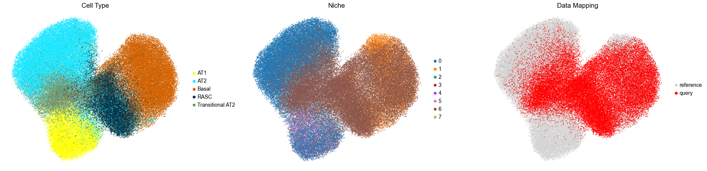
Reference
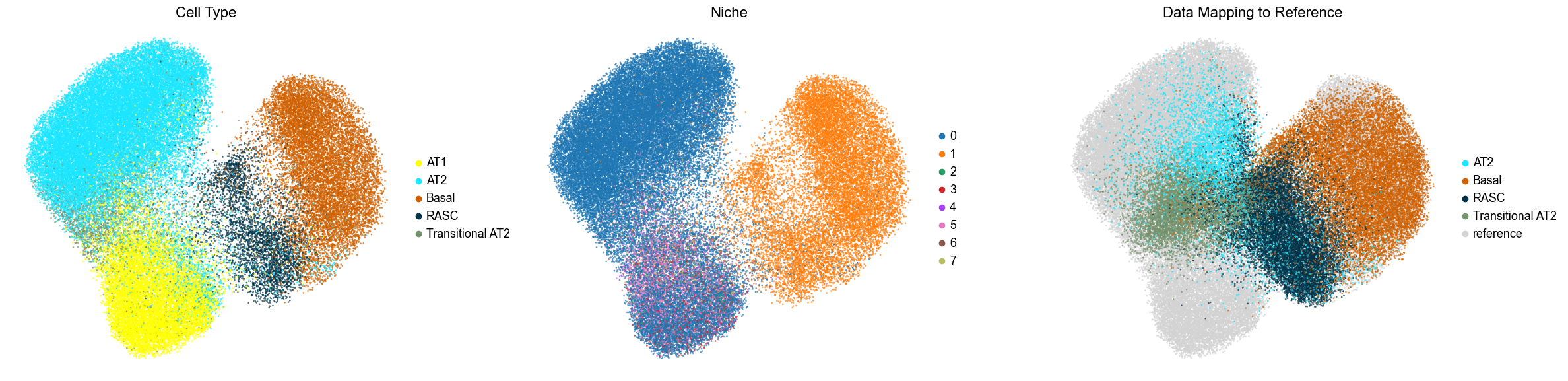
Query colored
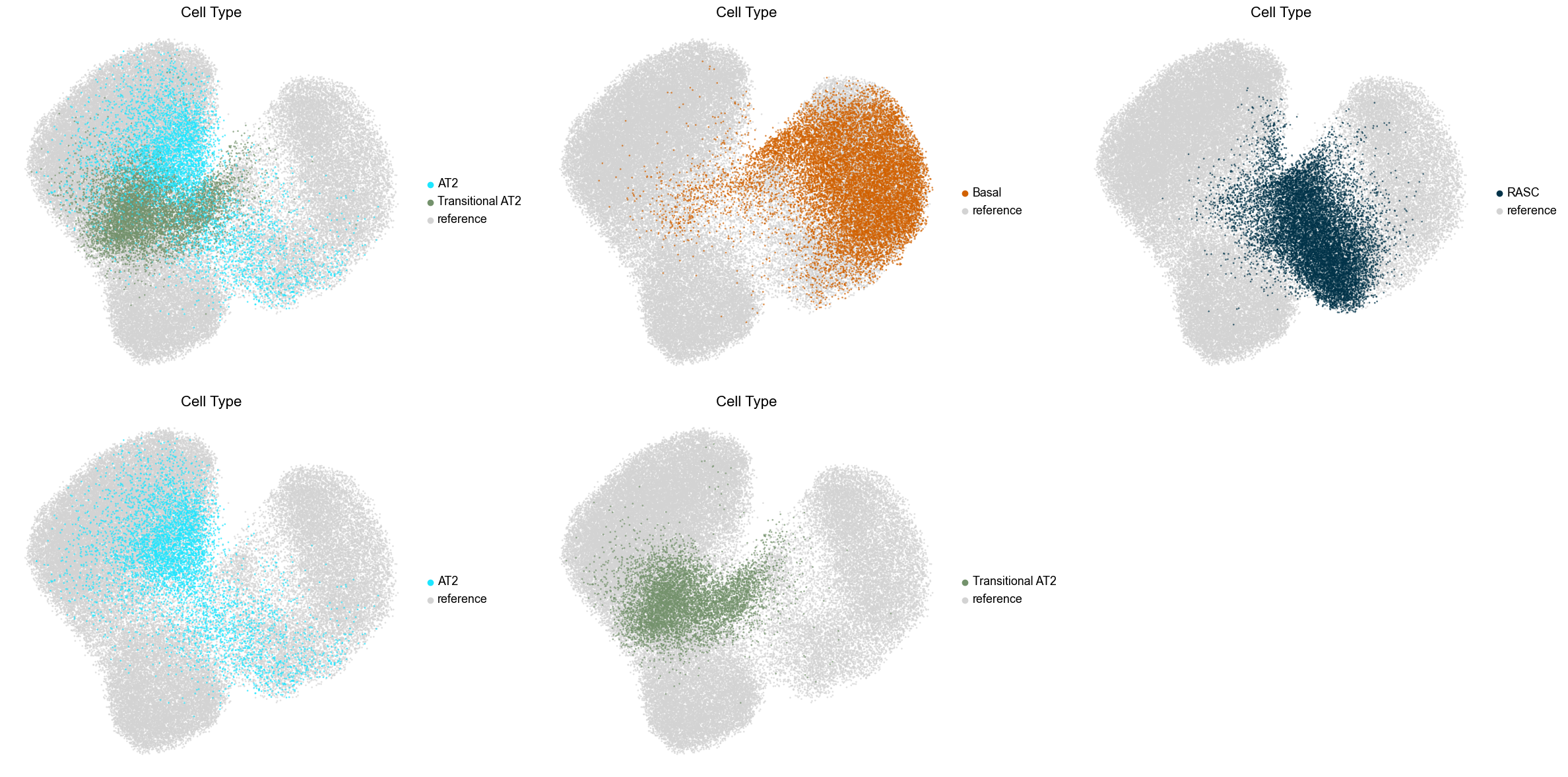
[77]:
from pyslingshot import Slingshot

adata_selected.obs['ct_name_used'] = [f"{adata_selected.obs['final_CT'][i]}_{adata_selected.obs['csn_label'][i]}" if
                                      adata_selected.obs['final_CT'][i] in ['AT2'] else adata_selected.obs['final_CT'][i]
                                      for i in range(adata_selected.shape[0])]
sorted(set(adata_selected.obs['ct_name_used']))
[77]:
['AT1', 'AT2_R2', 'AT2_basic', 'Basal', 'RASC', 'Transitional AT2']
[78]:
slingshot = Slingshot(adata_selected, celltype_key="ct_name_used", obsm_key="X_umap", start_node=2, debug_level='verbose')
slingshot.fit(num_epochs=1, debug_axes=None)
adata_selected.obs['pseudotime'] = slingshot.unified_pseudotime
Lineages: [Lineage[2, 1, 4, 3], Lineage[2, 1, 5, 0]]
0%| | 0/1 [00:00<?, ?it/s]
Reversing from leaf to root
Averaging branch @1 with lineages: [0, 1] [<pcurvepy2.pcurve.PrincipalCurve object at 0x000001F792ED5750>, <pcurvepy2.pcurve.PrincipalCurve object at 0x000001F7A2063AD0>]
Shrinking branch @1 with curves: [<pcurvepy2.pcurve.PrincipalCurve object at 0x000001F792ED5750>, <pcurvepy2.pcurve.PrincipalCurve object at 0x000001F7A2063AD0>]
100%|██████████| 1/1 [1:29:32<00:00, 5372.55s/it]
[ ]:
fig, axes = plt.subplots(1, 3, figsize=(24, 6))
axes = axes.flatten()

size = 15

palette = sns.color_palette("tab10", 6)
sc.pl.umap(adata_selected, color="ct_name_used", size=size, frameon=False,
           alpha=0.7, show=False, ax=axes[0])
for root, kids in slingshot._tree.items():
    for child in kids:
        start = [slingshot.cluster_centres[root][0], slingshot.cluster_centres[child][0]]
        end = [slingshot.cluster_centres[root][1], slingshot.cluster_centres[child][1]]
        axes[0].plot(start, end, c='black', linewidth=2)
        axes[0].scatter(start, end, c='black', s=30, zorder=5)
axes[0].set_title('Cell Type', fontsize=16)

sc.pl.umap(adata_selected, color="pseudotime", size=size, frameon=False, palette='viridis',
           alpha=0.7, show=False, ax=axes[1], colorbar_loc=None)
for root, kids in slingshot._tree.items():
    for child in kids:
        start = [slingshot.cluster_centres[root][0], slingshot.cluster_centres[child][0]]
        end = [slingshot.cluster_centres[root][1], slingshot.cluster_centres[child][1]]
        axes[1].plot(start, end, c='black', linewidth=2)
        axes[1].scatter(start, end, c='black', s=30, zorder=5)
axes[1].set_title('Pseudotime', fontsize=16)

sc.pl.umap(adata_selected, color="pseudotime", size=size, frameon=False, palette='viridis',
           alpha=0.7, show=False, ax=axes[2])
axes[2].set_title('Pseudotime', fontsize=16)

for j in range(len(axes)):
    axes[j].axis('off')
plt.tight_layout()
# plt.savefig(result_dir+"trajectory_withAT1_3.pdf")
plt.show()